292 | Optimising Your Tune With Histograms
Summary
Once we’ve completed the dyno tuning, it’s always advisable to confirm your tune on the road or racetrack. This can allow us to find small discrepancies between what we saw on the dyno in terms of air fuel ratio. We can then use histograms to quickly analyse a large amount of data and apply the required changes to the fuel or VE table. For this webinar we’ll be using MLVHD
| 00:00 | - Hey team, Andre from High Performance Academy here, welcome along to another one of our webinars. |
| 00:04 | This time we're going to be diving into the world of histograms. |
| 00:08 | We'll talk about what a histogram is, find out how we can use them and how they can be beneficial in helping to fast track our tuning. |
| 00:17 | Particularly when we are looking at analysing a lot of data. |
| 00:21 | Now when it comes to data analysis in general, there are a variety of ways that we can analyse or view our data and really depending on the data that we're looking at and what we're trying to achieve is going to depend on the best way of analysing or viewing that particular data so just as a really quick look here, let's just jump across to MegaLogViewer HD here and we've got a time graph which is probably the most common way most people look at data. |
| 00:53 | I'm going to come back and I'm going to analyse this in a little bit more detail as we go through the lesson, this is just a quick look at different ways we can have a look at our data. |
| 01:01 | So on the left hand side here, we've got the different types of data we've got available being displayed, so we've got RPM which is our red trace at the top, we've got our manifold absolute pressure which is our green trace and then of interest for this particular purpose we're looking at our air/fuel ratio, lambda compared to our lambda target so that's the data that we've got down the bottom in red and yellow. |
| 01:22 | This is quite a large amount of data though, this is from a drive out on the street with our Subaru WRX. |
| 01:31 | So it's hard really at a glance to take too much value from this and know how to analyse it, particularly if we are trying to find some trends maybe around our air/fuel ratio data. |
| 01:43 | Be very different if we had just looked at for example, just a single ramp run on the dyno. |
| 01:48 | There we'd have all of the data that we really need but here we're looking at multiple instances of the same situation in terms of manifold pressure and engine RPM. |
| 01:59 | And of course when we're looking at our fuel map in a speed density system, that's what we're mapped off so if we're looking at the same instances time and time again, let's say 3000 RPM and 85 kPa and we've got maybe 100 different samples through this entire file. |
| 02:14 | It's really difficult to see a trend so if we jump over here and again we'll have a look at this in a bit more detail, this is a histogram example and this shows us another way that we can analyse this data. |
| 02:26 | Won't dive into it in too much detail here and now because we'll learn a lot more about it. |
| 02:29 | But basically a histogram like this allows us to quickly and efficiently analyse a large sample size of data to find those trends that we need to understand in order to fine tune our calibration. |
| 02:48 | Now we can use the histograms for a wide range of different tasks as well. |
| 02:52 | Here I am talking about fuelling and that is probably one of the key areas that I use histograms a lot in my own tuning but it's definitely not limited just to that, we can use it for tuning our mass airflow sensor calibration, tuning our ignition timing if we're looking at knock events or knock retard which we'll look at as we go through today's lesson. |
| 03:11 | For the likes of HP Tuners and our GM tuning I also use this for dialling in some of our idle control target tables, our base airflow running tables as well. |
| 03:23 | Now as usual, as we go through today's lesson we will have questions and answers at the end so if there's anything that I talk about that you'd like me to explain in more detail, please hold onto those questions and we'll ask for those at the end so don't think you're going to miss out. |
| 03:37 | I'll just jump back across to my notes here. |
| 03:40 | Now the other aspect here is that we do need to understand that not every software package is going to give us the option of providing histograms. |
| 03:52 | HP Tuners with their VCM Editor software graciously did add that in and that's been a very powerful tool to fast track tuning in the GM/Ford world and basically any of the vehicles that HP Tuners support. |
| 04:06 | But a lot of software packages, data analysis packages for ECUs don't offer this but that's OK, that's where that MegaLogViewer HD package we've just had a look at a screen from. |
| 04:15 | That's relatively generic, pretty much as long as your data analysis or ECU software can provide a .CSV file, then you can import that into MegaLogViewer HD so again we'll look into that in more detail. |
| 04:30 | So let's have a quick tour here, or talk about HP Tuners which is going to be the first example of our user histograms here today. |
| 04:41 | And I've already touched on the common uses but essentially where I generally will use this would be for knock retard, for MAF calibration and for speed density calibration so what we'll do is we'll just have a quick look at HP Tuners VCM Editor software over here and this is our general layout, you can arrange the VCM Editor, sorry the scanner software however you see fit but basically on the left hand side of the screen here I've got the PIDs that we are looking at or the channels that we are looking at and that gives you a live value of that particular channel at a particular point in time. |
| 05:17 | I've got a logged piece of data here from a ramp run on our dyno so we can click at any particular point and obviously the channel will update with the relevant value at wherever I've put that cursor. |
| 05:29 | Next way of looking at this data is our chart versus time or time graph which we can see here. |
| 05:35 | So this, as I've mentioned this is a great way of analysing our data if we've done a ramp run which is exactly what you see here. |
| 05:43 | The red line on the screen at the moment is our engine RPM. |
| 05:46 | So ramp run here that I've just completed in 4th gear, we'll do this live as we move through today's lesson. |
| 05:53 | We can display any of the relevant channels that we're interested in. |
| 05:56 | Let's say we are looking here at our fuel tuning and we're trying to dial that in. |
| 06:02 | The two parameters that we're really interested in are displayed down the bottom here. |
| 06:07 | I am displaying these in units of lambda but in red we've got our commanded lambda, so this is the air/fuel ratio target or lambda target that the ECU is requesting at any particular time. |
| 06:18 | The green line that we've got in there, that is our measured air/fuel ratio so that's what we've actually got and that's coming from a wideband sensor fitted in the exhaust so at a glance here, we can do a pretty good job of seeing if there's any problems and we can see that for the most part, we're there or thereabouts. |
| 06:35 | If I click through this at a couple of points we can see that we're probably within about 1 or maybe 2% at worst, got a little bit of a lean spot here where we're 2% lean. |
| 06:44 | But we're pretty close, it's actually pretty well tuned which is a good thing. |
| 06:49 | Bit again this is a great way of analysing just a single ramp run but not so useful when we've got a large amount of data from a driver out on the street or if we're trying to maybe calibrate our mass airflow sensor calibration or perhaps our speed density sub system so let's just drag this out of the way and we'll have a look at how a histogram looks at least as far as the VCM scanner software is considered. |
| 07:14 | So this is our histogram or graph as VCM Scanner calls it and we've got a few here, some of these are pre configured and we can make our own which is one of the most common things we get asked about so we're going to go through that today. |
| 07:30 | But essentially the one I am on at the moment is one that I have created which is called EQ error, equivalence ratio error. |
| 07:37 | Basically how far off we are from our target air/fuel ratio. |
| 07:41 | So we've got this 3D table out here on the right hand side, we've got our manifold absolute pressure on the horizontal axis and we've got our engine speed on the vertical axis. |
| 07:50 | This was for that ramp run that you've just looked at so we've got a few pieces of data here which are really captured from the overrun area where I've backed off the throttle or where we've gone through to full throttle at the start of the run. |
| 08:02 | These aren't really relevant here but what we've got here is the data that we've captured during that wide open throttle ramp run. |
| 08:09 | I will talk a little bit more about what these numbers mean and how we can generate these but essentially this is how close we are to that target. |
| 08:18 | You can see that for the most part we're pretty good there. |
| 08:22 | Basically we're within 1-2% of our target the whole way through. |
| 08:26 | Red numbers which we've just got this little area here 0.8 and 0.6 which are a little bit tinge of pink there, those mean that we are leaner than our target. |
| 08:35 | Whereas the green shading here, 1.8, -2.3%, that means that we're richer than our target. |
| 08:42 | I like to do this colour coding here because at a really quick glance I can straight away see if we are safe or maybe if we're moving a little bit lean, that could be problematic, just gets me a visual guide straight away and very quickly as to what the situation is and what the magnitude of that error is. |
| 09:03 | The further we get away from our target the more brightly coloured these will become which is why we can see here we've got -15 to -20% here, we've got really bright greens and likewise you can see there we've also got some bright red where we have the large positive errors. |
| 09:24 | I'm just going to get my doc open here as well so that we can carry on, bear with me. |
| 09:35 | Should have started this before the webinar but we'll get there. |
| 09:41 | No we won't. |
| 09:43 | Never mind, we won't do that, I'll just head back across to my notes for a second. |
| 09:48 | Alright so what we need to actually, oh actually no sorry I wanted to also show you a couple of the other histograms that are available so by default you'll always have with the factory installation, the generic installation of the VCM Editor Suite, you will have these two histograms that are shown up the top, so we've got spark advance and spark retard. |
| 10:14 | Now these are quite useful for a couple of reasons. |
| 10:16 | First of all we can use the spark advance tab to physically see where abouts we were accessing inside the spark table. |
| 10:26 | That's important particularly because the axis for this table is cylinder air mass. |
| 10:34 | Which isn't particularly useful for a lot of us trying to decide what our cylinder air mass in grams per cylinder was when we were running the car. |
| 10:44 | If we're running on a speed density subsystem on an aftermarket ECU, usually this is pretty easy because we are using manifold absolute pressure so if we're naturally aspirated we're going to be probably 95 to 100 kPa there or thereabouts during a ramp run so we know where abouts we're operating in the table. |
| 11:00 | As you can see with this, it's not that straightforward, we start here at the start of the run, 1600, 2000 RPM, 0.64 grams per cylinder and then we move down at higher RPM where the volumetric efficiency improves, we move down to around about 0.88, 0.90 grams per cylinder before dropping away again so what we can do, we head across to our VCM Editor, let's just move over to our spark tab. |
| 11:28 | And then we can move down to our base high octane tab which is where we're going to be doing the majority of our tuning. |
| 11:35 | And what we can see is that first of all, the axes spark air mass on the vertical and spark RPM on the horizontal, those match the values in our table here. |
| 11:47 | The break points don't, don't worry about that, I'll explain that in a second but the actual axes do so what that means is we can see that again, start of our run, we were 0.64, 2000 RPM. |
| 11:59 | So we can correlate that across and we know that we were 0.64, 2000 RPM so we're around about here. |
| 12:08 | So it lets us just know exactly where abouts we are in the table and what this is important for is it allows us to know if we're going to make some changes to this table, where exactly we want to make those changes. |
| 12:21 | Now the other aspect, again if we head back to our editor, our scanner I should say, spark retard. |
| 12:26 | Now I don't have any knock present in this particular log file. |
| 12:30 | I'll quickly have a look, it might be a bit too hard to find at a glance but I'll quickly have a look. |
| 12:36 | I think I should have a knock file. |
| 12:41 | If I do, here we go. |
| 12:45 | So I'll just quickly load this up. |
| 12:47 | So this is another log file that we've created with the same car and if we look through this log, OK start of a ramp run here, you can see these large spikes in red, these are our knock retard so this is where the ECU is noting detonation and it's pulling timing. |
| 13:09 | At the point that I've just put the cursor there, we can see that it's pulled out 9.5° of ignition timing. |
| 13:14 | So what this means is that our base calibration, our base timing, possibly a little bit optimistic there, a little bit over advanced so again if you've got a lot of data, particularly if you're looking at cruise data, it can be difficult to pinpoint exactly what cells in the spark table you need to modify, I'll drag this back down. |
| 13:32 | By looking at our spark retard histogram we can see exactly where that was occurring. |
| 13:37 | So we've got 4° knock retard there at 1200 RPM, 0.64, 0.68 grams per cylinder. |
| 13:45 | Got a little bit more happening down here as well so this just gives us a quick guide on where we need to make those changes. |
| 13:52 | Now if you've been out for a drive on the road and you've got a lot of data, you're going to have filled in a lot of this area of the table as well. |
| 14:00 | And again, that's going to be very quick and easy to identify where abouts you have that knock retard occurring. |
| 14:07 | So making it quicker and easier to fine tune your actual spark tables. |
| 14:12 | Alright we'll just head back across to my notes here for a second. |
| 14:16 | Important just to talk about what inputs you are going to need, how you're going to need to be able to capture that data. |
| 14:25 | And the first one is pretty obvious, if you're looking at fine tuning your fuel you're going to need a way of comparing the commanded or target air/fuel ratio to your measured air/fuel ratio. |
| 14:36 | So of course we're going to need a wideband air/fuel ratio meter and we're going to need to scan that parameter. |
| 14:41 | Now if you've got an aftermarket ECU, while it's definitely not an absolute essential, these days, particularly given the relatively low cost of a wideband controller, I almost always end up with those installed, if possible I'm going to be using a CAN based wideband controller and that's going to send the wideband air/fuel ratio data directly into the ECU via CAN where it can be logged. |
| 15:06 | You can also use it in some ECUs for auto tuning or you can also use it for logging. |
| 15:12 | So that gives you the input that you need to compare to your target. |
| 15:15 | In the case of reflashing here with the Gen 4 GM LS, in this case it's an L98 that we've got, the factory air/fuel ratio sensors are only narrowband so they're essentially pretty useless to us for our purposes of tuning, particularly under wide open throttle. |
| 15:36 | So we've got an AEM X Series wideband and why I quite like that sensor, that controller is that it does output that data through an OBD2 passthrough onto the CAN bus. |
| 15:50 | A bit of a mouthful, basically all that means is it's going to output the wideband air/fuel ratio data via a CAN message. |
| 15:57 | The HP Tuners VCM Scanner software is set up to be able to understand that information and why that's really nice is it's a clean quick and easy way of getting that data into the scanner and unlike an analog voltage based air/fuel ratio meter, there's no chance of the data being affected by ground offsets so we're guaranteed the robustness of that data and of course when you're relying on air/fuel ratio data you want to know that you can trust that. |
| 16:24 | If you are going to be looking at using knock retard, that's a function or an input that is already, a channel that's already being logged via the VCM Scanner software if you are tuning GM so that's nice and easy, you don't need any additional setup in there. |
| 16:41 | Now the other thing that is quite important here is if you're tuning the fuelling you are going to need to have a math channel that gives us the difference between our target and our measured air/fuel ratio so for those of you who have gone through our EFI Tuning Fundamentals course, for me one of the key takeaways from that course is the ability, the understanding of how to quickly in one shot correct your air/fuel ratio from what it's actually being measured at to correct it to a target and for those of you who may remember that, the formula we use there is our target, our desired, sorry the measured air/fuel ratio, so the air/fuel ratio we actually have, we divide that by the target or desired air/fuel ratio, the air/fuel ratio we want and that will give us a correction factor and then if we multiply the actual fuel table value, and that doesn't matter whether it's a MAF frequency or it's a speed density, volumetric efficiency number, if we muliply that by the correction factor, it's going to get us onto our target. |
| 17:45 | So really what we want to be able to do is quickly create that math channel for ourselves. |
| 17:50 | Now in the case of HP Tuners, they actually do this for us. |
| 17:55 | Provided we have a wideband connected there is a predefined math channel in HP Tuners VCM scanner that will give us that output so again if we go down to our equivalence ratio error, this again is a file that I just loaded up as you watched me so it's not the one that we originally saw. |
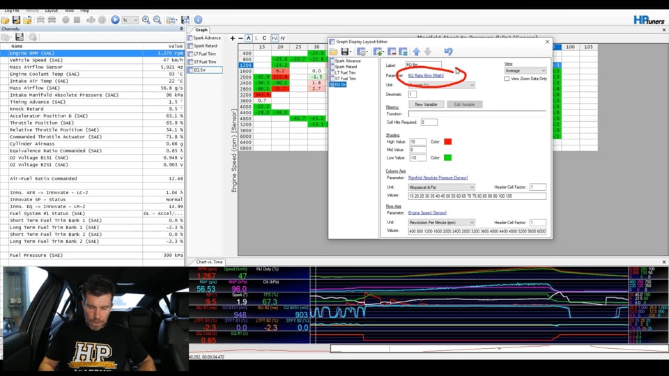
| 18:16 | But the data in here is our equivalence ratio error and what we'll do is we'll just quickly right click here and we'll go to our graphs layout and we'll see what that actually is. |
| 18:27 | So we want to come down to the particular histogram that we want to edit here which is our equivalence ratio error and the parameter that we are logging in here is equivalence ratio error and you can see in brackets there it says it's a math channel. |
| 18:41 | So this is predefined and I'm going to go through and show you how to set this up. |
| 18:46 | And all it does, you can make your own if you really want, all it does is it basically does the calculation we've just talked about. |
| 18:53 | Looks at the measured air/fuel ratio, divides that by the target air/fuel ratio and then expresses that as the percentage so that gives us our error. |
| 19:01 | Why that's really important is that if we've got that data represented in this way, we can actually use the data in our histogram and paste that correction factor directly into our speed density or our mass airflow sensor calibration tables. |
| 19:15 | Alright a lot of information to take in there and I know this is probably still confusing so what we're going to do is have a look at how we can actually set up some histograms. |
| 19:24 | We're going to look at 2 here but basically the technique that I'm going to go through, the process, you can apply to just about anything you're interested in setting up a histogram for, regardless if you're looking at idle airflow or speed density, it doesn't matter. |
| 19:41 | So let's have a look first of all at setting one up that we would use to help us calibrate our mass airflow sensor. |
| 19:48 | So if you're running a conventional stock engine which still relies on the mass airflow sensor, that is the main load input so that's obviously something we really need to get set up. |
| 19:58 | So what we'll do is we'll start by heading across to our VCM Editor. |
| 20:03 | Let's just have a look at what that mass airflow sensor calibration actually looks like. |
| 20:07 | So what we want to do is start by heading over to our airflow tab. |
| 20:10 | And our MAF calibration airflow versus frequency is what we've got here. |
| 20:15 | So let's click on that. |
| 20:17 | And we've got a pretty simple table, 2D table here, the break points or axis for this table is the frequency output from the mass airflow sensor. |
| 20:26 | So this is what the ECU is actually measuring. |
| 20:30 | The frequency that the mass airflow sensor is outputting. |
| 20:32 | And this table essentially converts that frequency into a mass airflow. |
| 20:37 | And in this case we're representing this in grams per second but doesn't really matter the units. |
| 20:42 | So essentially what this means is if we were seeing a frequency at the ECU of 8400 Hz, that would mean that we have 162.96 grams of airflow per second. |
| 20:57 | We've got this represented graphically as well and I mean aside from our histograms which is the topic today, a well tuned mass airflow sensor calibration should have this nice smooth exponential shape. |
| 21:10 | Alright so that's the table that we're going to want to fill in. |
| 21:13 | When we're doing this, again what we're trying to do is calibrate this so that essentially our measured air/fuel ratio matches our target. |
| 21:23 | If that's the case, provided of course that our injector data is accurate and correct then that should mean that our mass airflow sensor calibration is also correct. |
| 21:32 | Alright how do we use the scanner to do this? Well let's have a quick look at this. |
| 21:37 | So we don't actually have a MAF calibration histogram here to help us which is absolutely fine because that's where a lot of you will be starting from so what we can do is create one. |
| 21:47 | We're going to start by clicking on add graph. |
| 21:50 | And we'll click add table so what we want to do is give it a label, just so we know what we're looking at when we come back to this at a later point. |
| 21:59 | So let's call it EQ error and we'll call it MAF. |
| 22:03 | Now the first part here is what parameter are we actually interested in logging into this? So again, what are we trying to do? Here we are trying to optimise our fuelling so of course we want that parameter we've already talked about, equivalence ratio error. |
| 22:20 | So let's click on that and start. |
| 22:22 | Now there's a huge list here of all of our options and there's a variety of different ways of actually finding the parameter we're interested in. |
| 22:29 | We can click through, in this case we are looking for our math channels so those are all down here. |
| 22:37 | So we can click through and in this case lambda and air/fuel ratio, we will find those down here. |
| 22:45 | So EQ ratio error, that's what we want. |
| 22:49 | We can click on that and I'll just point out here, we have 2 options here, we've got equivalence ratio error and we've got air/fuel ratio error. |
| 22:56 | Essentially they're giving us the same thing but which one you want to choose is going to depend on how you are representing your target equivalence ratio and your wideband data. |
| 23:06 | If you are presenting these in air/fuel ratio units then you will use AFR error. |
| 23:11 | Otherwise if like us you're using lambda, you'll use EQ ratio error. |
| 23:16 | So that's how we would choose that. |
| 23:19 | The other way of doing this is if we're not quite sure exactly where we find it, we can just start typing. |
| 23:24 | So if I type equivalence ratio, obviously I can complete that. |
| 23:29 | We can start to see everything that is relevant to what we're trying to look for here and again, we scroll down the bottom, we've got EQ ratio error. |
| 23:37 | OK so that's the one that we want. |
| 23:39 | Now the unit here is already auto filled, it is a percentage which is what we want, we can also choose how many decimal places that we want. |
| 23:47 | In this case 1 decimal place is probably absolutely fine. |
| 23:52 | We can also choose to add some filtering in here. |
| 23:57 | Now this isn't something that I use a lot in the VCM Scanner software. |
| 24:01 | Simply because when I am using this software, 9 out of 10 times I am on the dyno where I have a lot of control over the way the car is being driven. |
| 24:08 | But if you're out on the street that may not be the case so we'll have a look at this further on in MegaLogViewer but essentially you could filter out for example areas where you don't want data being logged, maybe at cold engine temperatures or at closed throttle so depending what you're actually trying to achieve there. |
| 24:27 | Now we can add some shading here so let's say if we've got a high value, let's say we're going to call a high value 10 and we're going to call a low value -10 and again we can start to choose a colour for these. |
| 24:41 | Let's say if it's a high value we're going to go red and if it's low value we're going to go green. |
| 24:46 | Absolutely no requirement to do this, this is personal preference, however you want to set it up. |
| 24:52 | As I said already, for me this just gives me at a glance a bit of an indication of the magnitude of error that we've got. |
| 24:59 | Alright so now the important part, we need to choose the column and row axes. |
| 25:04 | So in this case remember we were only looking at a 2D table so it is a horizontal table so we're looking at our column axes. |
| 25:13 | And what we want to do is click on this and choose our parameter. |
| 25:17 | Before we do that, let's just dive back to our editor. |
| 25:20 | We can see here that the parameter we're going to be looking for is our mass airflow sensor frequency. |
| 25:25 | Let's head back and we will find that, so we click on choose parameter. |
| 25:29 | Again we can just start typing and it will auto fill so not particularly difficult. |
| 25:34 | Everything related to mass airflow pops up and we want frequency. |
| 25:39 | So it's important to choose the frequency one here. |
| 25:42 | Double click on that and that will give us the parameter that we're interested in. |
| 25:47 | Last part of the process here, we need to choose the break points. |
| 25:52 | This is really important because if the break points for our histogram don't match the ones in our editor, that's going to give us some value, some data but it's not going to make it possible for us to use the correction, the copy and paste of the percentage error to automatically correct our table so let's just dive back and we'll show you how easy that is. |
| 26:14 | We don't need to go through and copy each of these down. |
| 26:18 | If we simply right click here, we come down to column axes and we click on copy labels. |
| 26:23 | That's going to copy all of these X axis break points here onto the clipboard. |
| 26:28 | Head back across to our editor, come down here into values, right click, paste, job done. |
| 26:36 | Alright so that's created our EQ error, I'll just relabel that MAF. |
| 26:41 | That's created our little histogram now so we can close that down and we can see that pops up in the left hand side here. |
| 26:48 | Let's click on that and what we'll do now is we'll just get our data closed down and I'll just start the car up. |
| 26:57 | Now you'll have to bear with me here, this car unfortunately is running a speed density patch so it doesn't have a mass airflow sensor anymore so what this is going to do is pin us at 0 frequency but let's just get ourselves recording and we'll see what actually happens there. |
| 27:15 | Now at the moment everything is warming up so we have a bit of an error showing but we can see we're sitting at a frequency of 0, we can see that our air/fuel ratio being measured at the moment is sitting at 1.09 so we do have an error there. |
| 27:31 | As everything warms up that's going to come down and you can see that value is slowly but surely, started up in the 20s, now we're down at 10%. |
| 27:40 | Now of course if we did have a mass airflow sensor fitted on this car, as I blipped the throttle and we moved around, we would be moving all around this table, that's not he case because we have a speed density patch applied but essentially if you've got a mass airflow sensor, the job is done. |
| 27:56 | Let's have a look at something a bit more relevant to this particular vehicle though, we will, I'll just get our fan up and running here so we don't end up cooking the engine bay, let's have a look at how we can set up our equivalence ratio error for our speed density. |
| 28:10 | So again we'll go through exactly the same process, this might be a bit of a rinse and repeat and it really is but we get quizzed so often on how to do this, I just really want to give you the tools so that once you understand this, you can apply it irrespective of the type of histogram you're trying to create. |
| 28:25 | So let's close down our mass airflow sensor frequency and we are running this speed density patch so what this does is it gives us 3 volumetric efficiency tables here. |
| 28:36 | And these are IMRC open and closed and VE displacement on demand. |
| 28:42 | Basically in our instance we make all 3 the same so let's just have a look at one for an example. |
| 28:47 | We've got the table set up here. |
| 28:49 | Looks like a conventional speed density table that we'd see in an aftermarket ECU only the numbers inside this table we can see that we're in the high 2000s in some areas. |
| 28:59 | So this is GM VE. |
| 29:01 | The numbers, not 0-100% like we'd normally expect but it still works in exactly the same way. |
| 29:07 | Alright so let's go through the exact same process, let's have a look at what we've got here. |
| 29:11 | So on our X axis we've got our manifold absolute pressure. |
| 29:14 | On our vertical axis we've got our engine RPM. |
| 29:17 | No problem. |
| 29:19 | Let's head back over to our scanner. |
| 29:20 | So we already have this equivalence ratio error histogram set up but let's just pretend that we don't. |
| 29:29 | So we'll go and we'll delete that. |
| 29:32 | And we're going to add another one, add table and basically this is going to be very similar. |
| 29:39 | So we'll call this EQ error SD and we need to click for our parameter. |
| 29:45 | Again this is going to be the same one that we've already looked at, equivalence ratio error so so far so good. |
| 29:51 | Alright double click on that and again I'm quite happy with 1 decimal place there. |
| 29:56 | We're going to set our high value to 10 just like we already did, our low value to -10 and we'll set the same colour coding here, just to give us a bit of a quick visual cue. |
| 30:07 | OK so now we're onto the more important stuff, setting up our column and row axes so for our column axis, let me head back over to our editor, we know that our column axis is going to be manifold absolute pressure. |
| 30:20 | While we're here let's just speed this up a little bit, we'll go to column axes and we can click on copy labels and again if you don't remember, you can do that just by right clicking anywhere on the table, go down to column axis and copy labels. |
| 30:32 | Alright let's head back over, we want to click on our parameter and we want to enter manifold, if I can spell this right. |
| 30:46 | Absolute pressure. |
| 30:48 | And we can click on 1 of these elements, that's going to give us the correct PID, the correct channel. |
| 30:58 | Then we click on our values, control V or right click and paste, job done. |
| 31:02 | OK row axes, we know that that was engine RPM so we can click RPM, we'll click on our engine speed. |
| 31:12 | And we can go back across to our editor. |
| 31:16 | Again right click anywhere on the table, row axis and copy labels, back across to our scanner, right click and paste and our job is done there so we close that down and again I'll just change that back to SD so that we can distinguish between those two. |
| 31:33 | So now we've got our SD error table so we can see straight away, we've got these same break points, we're sitting there at idle at the moment and we're clicking away at 65, 70 kPa, again we've got a pretty large cam in this and we've got our error sitting at 2, 3%. |
| 31:49 | Let's got through and gather some data and we'll talk about some of the ways we can gather this data and what's important when we are using a histogram to gather data. |
| 31:56 | We can do this 2 ways, we can use the histogram with saved data, with logged data which is what we looked at before, or we can gather it live and what we'll do is we'll just get ourselves up and running here on the dyno and what we want to do before we start logging our data is we want to make sure that we're gathering good quality data, just like anything, basically using a histogram is a case of garbage in, garbage out so we want to make sure for example that before we start gathering our data that our engine is up to normal operating temperature and we also want to make sure that we aren't suffering from heat soak. |
| 32:30 | This is a really common trap, particularly when you're reflashing a factory car because the process generally if you're out on the street or on a racetrack will be, you'll gather some data, then you'll pull over to the side of the road, analyse your data and make changes, flash those in and then start the car up and drive away again. |
| 32:48 | Over those maybe 2-5 minutes that you've been sitting there, the engine bay is going to become heavily heat soaked so for the first couple of minutes, while we're out there driving, we're going to be affected by that heat soak and that's going to in turn affect our results so we want to make sure that we're getting good quality data, get rid of that heat soak, so if we're doing road tuning, always drive the car for 2-3 minutes, get rid of that heat soak, get some airflow through and then you can start logging data. |
| 33:14 | So you can see at the moment we've gathered some data and we have probably got that situation going on here so what I'm going to do is simply stop logging and I'm going to start logging again. |
| 33:24 | Alright so what we can see here, at the moment I'm sitting at 1400 RPM just barely ticking along at 50 km/h and we're sitting between 55 and 60 kPa and the numbers are looking pretty good. |
| 33:36 | Got an error of about 1.5, 1.3%. |
| 33:39 | I am cheating a little bit here and this is really important to understand. |
| 33:44 | At the moment I do still have our closed loop fuel control enabled so if we look over here on the left hand side, we can see that we've got our short term fuel trim for bank 1 and 2 ticking away there and they're sitting between about -2 and -5% so there or there abouts, probably not quite ideal but it's important to understand that when we are actually doing this, as opposed to just my quick demonstration here, what we would do is put the engine either, put the ECU either into open loop mode, so that would be ignoring that closed loop trim, nothing would happen, and then we're actually seeing the real error that exists between our target air/fuel ratio and our measured air/fuel ratio. |
| 34:22 | Alternatively if you do leave the short term fuel trims enabled, you would need to change your math function so that it incorporates the correction into your calculation. |
| 34:32 | So just important to mention, at the moment we're not seeing a true representation of this error because of our closed loop. |
| 34:38 | As long as we understand that though it's perfectly fine for our demonstration. |
| 34:42 | So let's gather some data here and what I want to do while I'm doing this is be nice and smooth on the throttle, get as many hits in the cells as possible and why I want to be smooth on the throttle is just to make sure I don't bring in any acceleration enrichment or any decel enleanment. |
| 34:57 | So those can affect our accuracy. |
| 34:59 | So regardless whether you're out on the road or on the dyno like I am here, just pays to be nice and smooth on the throttle and as consistent as we can. |
| 35:08 | And as we move around here, we can see that we're up to 1600 RPM and 70 kPa You can see as I go into a new cell, let's do this now, we'll go up in the throttle, we'll go up to 75 kPa, 80 kPa, generally what we'll find is that when we move into a new cell, initially we'll start to see it populate and then we might see the numbers change a little bit so I'll just bring the RPM up. |
| 35:30 | And what we want to do is we want to stay in a cell long enough that we see the number stabilise 'cause what we're actually doing at the moment is we're looking at the average of every hit we get in that cell so as I'm talking here, we're sitting at 1800 RPM, 70 kPa, 100s of times every second the scanner is looking at the data and it's taking a measurement of how far we are from our target and it's updating that. |
| 35:57 | So we're pretty stationary at the moment which is good. |
| 35:59 | Let's increase our throttle opening, we'll gather a little bit more data here. |
| 36:06 | And let's bring our RPM up, we'll do the same at 2000 RPM here. |
| 36:11 | So again just nice smooth changes to our throttle position, nice smooth changes on the dyno RPM set point as well and we want to basically fill this histogram in, gathering as much data, hitting as many cells as we can. |
| 36:25 | Now I'm just going to stop the recording here and back off because essentially the process is exactly what you've seen. |
| 36:31 | We're not going to sit here for the next half hour filling this table in but let's have a look at what the data means. |
| 36:36 | So first of all, again not withstanding the fact that we are in closed loop mode, we can see that these numbers, we'd all be pretty happy with that, generally if we're within about +/- 2-3%, I'm pretty happy with the calibration and that's exactly where we are, no surprises there with our closed loop active. |
| 36:55 | But we want to know what the numbers actually mean and whether we can trust them here so that's where we can look at these little values here. |
| 37:04 | So at the moment we've got this little A box highlighted and this stands for average value. |
| 37:08 | So this, as I said, every time we're sitting in a cell, the ECU is logging data continuously and that A means that we are averaging all of the hits in that particular cell. |
| 37:19 | Why that's important is that it allows us to average out and remove any outliers that really aren't that relevant. |
| 37:27 | And gives us a true indication if we've got a lot of good quality data, what the actual calibration is like for that particular cell. |
| 37:34 | To get a bit of an idea of how much we can trust that data, we can come over and click on the C button there which gives us a count, it tells us how many individual counts we've had of data for a particular cell. |
| 37:46 | So we can see in the middle here where I was sitting for a little while, for 1800 RPM and 70 kPa, we've got 1100 hits. |
| 37:53 | Obviously it's a lot of data, we can be pretty confident that that data's going to be accurate and we can trust it. |
| 37:59 | However we've got a couple of little outliers here, 2 and 5 hits, we've just had a bit of a flash in the pan where we've jumped into that cell and we haven't really got solid data. |
| 38:07 | Obviously with so few counts I'm not going to trust that data too implicitly. |
| 38:13 | Now again just to compare this back, let's jump across to our MegaLogViewer HD and our actual time graph and this is what I was talking about, it's really hard when we're looking at this comparison in a time graph of our measured air/fuel ratio versus our target's really hard to really see am I too rich or too lean at let's say 2000 RPM and 70 kPa? We can't see at a glance every time we were in that cell but when we go over to our histogram, that gives us that indication so really good solid data. |
| 38:47 | Alright what we'll do as well is we'll just quickly have a look at how this can be used for a ramp run. |
| 38:53 | Now what I like to do when I'm going to do a ramp run is I like to make sure that I am only gathering data that is relevant to the ramp run and we can do this by making sure that we only start the logger when we are at full throttle, just before the ramp run and we can turn it off or stop it before we back off the throttle. |
| 39:14 | That's not to say it's the only way of doing it but it just does make sure that we have nice clean data. |
| 39:19 | So what we'll do, we'll head over to our dyno for this one here and we'll get ourselves up and ready to run and I'll just make this run in 4th gear here. |
| 39:32 | And we'll just get the dyno ready to settle, actually I will gather some more data just so we've got a full understanding of this. |
| 39:42 | Alright we're at full throttle here, we'll click on OK and we're obviously just going to be plotting our power graph here, we'll have a look at our actual results in a second. |
| 40:02 | Alright so let's just have a look, first of all, 452 horsepower at the wheels so reasonably solid result here. |
| 40:11 | Let's jump over to the laptop screen again and we can have a look at our time graph here and again we've got our measured lambda versus our target. |
| 40:21 | So in this instance it's not a bad way of making our changes, we can see exactly what's going on from this data so for example what I mean by that is when we're looking at this data it's only passing through 1 RPM zone once obviously so we've not got that situation where we're out on the road where we've got multiple instances of a certain combination of RPM and load. |
| 40:42 | So let's say here we're looking a little bit lean, 0.89 target, 0.93 measured so we know that in this instance, 3500 RPM and 94 kPa, that is the cell in our editor that we would want to actually make changes to. |
| 41:00 | But we should also have, if we bring this down, go back to our table here. |
| 41:07 | That's interesting. |
| 41:11 | It's displayed the numbers in a not particularly useful way to us, not actually quite sure what's gone on there but what we should have is the data showing us again exactly where we are operating at wide open throttle. |
| 41:23 | Now again I did talk about the fact that we want to be careful how we measure our data and I did end up pressing record before I went to wide open throttle just to show you that, so you can see we've got this transition up here to wide open throttle and we also have the area where I sort of backed off and got back down to closed throttle. |
| 41:44 | Now this can upset our results if we're going to use the entire data for a copy and paste. |
| 41:50 | So that's why I want to be careful with that. |
| 41:53 | Let's just get our logger up and running again and not quite sure why we are getting useless data at the moment, so let's go back down to our speed density error. |
| 42:08 | Interesting. |
| 42:10 | These are the sort of things that happen when we do our webinars live so let me just try and get that corrected, I don't know what has changed because it was doing a really nice job of demonstrating exactly what it should look like as you all obviously saw. |
| 42:26 | Let's close that down and see where we are. |
| 42:29 | Oh I know exactly why it's because I'm still on count. |
| 42:33 | OK so I've just ruined that data but that's OK. |
| 42:37 | Now what we, so if I go back to our average values, that would have shown us essentially what we had in our graph, so trap for young players, make sure that you are on average when you are actually trying to make use of the data. |
| 42:52 | Now the other thing we can do here is once we've got a lot of data selected or a lot of data created, the power of this, which I have mentioned is we can highlight all of our data here and we can right click and click on copy and if we've got all of this data where we've got some errors being represented, what we can do is come back into our editor and we can right click, we can highlight the table, right click and then if we come down to paste special, what this allows us to do is make automatic corrections to this table, so this is a speed density table, matches our break points for our histogram, what we can do here is basically choose this multiply by percent. |
| 43:33 | What that's going to do is automatically apply the error from our histogram into this table. |
| 43:39 | In this case I'll click on that and it's only obviously made a very small change there because that was exactly what we had data logged for. |
| 43:49 | So in this case, what we can see, it's showing red, we know that means it's lean, in this case essentially we're looking at about 3% lean and if we go back to our editor, what it will have done there is applied a 3% positive change to these cells. |
| 44:02 | Adding 3% to our volumetric efficiency which should correct that error. |
| 44:06 | So there's a really fast way of using the histogram to collect a lot of data and then automatically using that data to correct our VE table, our speed density table. |
| 44:16 | However as I mentioned, it's very much a case of garbage in, garbage out so we do need to be mindful if we are looking back at the logged data that we have in here and you've got numbers all over the place or you've got a lot of individual cells where you've only got one or two hits in those cells and we can't really trust the data, it's going to blindly apply those corrections so I'm always very cautious with this. |
| 44:41 | I will generally use a bit of common sense here and if we've got a nice smooth trend to the errors that I've got, and I've got a lot of hits, a lot of counts in each of the cells, then I can trust that data, I'm going to be confident using the paste special function. |
| 44:59 | If not though, if I've got some really big outliers, I would be more inclined to use a bit of manual blending and do the adjustments by hand, it really just comes down to the quality of your data, I will just come back to the editor and point out one more thing though. |
| 45:15 | You also have, under paste special, multiply by percent half. |
| 45:20 | So does exactly what it suggests, instead of applying the full correction that we just calculated in our histogram, it'll apply half of that. |
| 45:27 | So generally once you're getting close to your target, using this can be an easier way of creeping up on it and generally within 2 or perhaps 3 iterations you should have your speed density table or your mass airflow sensor calibration, whichever you're optimising, pretty well dialled in. |
| 45:44 | Alright so that covers off the HP Tuners side of things as far as we're going to go here. |
| 45:50 | If you've got questions, probably now is a good time to start asking them, we'll just go through a quick demonstration on the MegaLogViewer HD which we've already had a quick look at and then we'll jump into those questions so if you've got questions, ask them now. |
| 46:05 | Alright so the MegaLogViewer data, as I've mentioned, MegaLogViewer is helpful because it'll work with basically any .CSV file. |
| 46:12 | So as long as your datalogger or ECU can generate a .CSV file, you're golden. |
| 46:18 | So let's have a quick look, the particular ECU that we were using for this demonstration was the Ecumaster EMU Black fitted to our Subaru STi and here is our volumetric efficiency table. |
| 46:34 | So it's kind of much the same although there's a little bit more work involved in actually setting up the histogram so we can see there on the vertical axis we've got our RPM, on the horizontal axis we've got our manifold pressure and we can take note of the break points. |
| 46:48 | Head over to MegaLogViewer HD and I've already got this log file loaded up. |
| 46:53 | One little trick with Ecumaster is depending on the parameters you've got loaded up on the logging in the ECU, that is the parameters that will be logged so unfortunately in this instance, I hadn't selected throttle position so that's not available here and why that's important is it does affect our ability to filter the data. |
| 47:16 | We've got our log viewer, our time graph pretty much, I already talked about that so we'll head back over to our histogram and table generator. |
| 47:25 | Obviously MegaLogViewer HD is very much tied into the MegaSquirt range of ECUs so there's some functionality that is very very quick and easy to use with MegaSquirt but that's not to say it's the only software that you can use it with. |
| 47:41 | So what we'll talk about is how this is set up and first of all, to do this we've got our axis fields here. |
| 47:48 | Kind of pretty much the same as what we've already looked at. |
| 47:51 | We've got our X axis as manifold pressure and our Y axis as RPM. |
| 47:55 | You can choose from the available parameters that were logged by click on the list, I'm not going to change that. |
| 48:01 | So that basically just allows us to then set up these axes and then much like we saw with the HP Tuners VCM Scanner software, we then need to manually adjust this time the break points on each of these axes so that they match. |
| 48:20 | Now we can't necessarily copy and paste the error in this case but it's always nice to have those break points at least pretty close so we can at a glance see exactly where we were in the table so we'll just jump back over to our Ecumaster software and we can see that those break points do in fact align with what I've got in this table. |
| 48:40 | Alright coming back to MegaLogViewer HD. |
| 48:42 | The key one here is, just try and get out of that, the Z axis. |
| 48:49 | So in this case, you can see that the parameter I've got here, is called ECU M AFR. |
| 48:55 | Now this is actually a user channel and it's essentially again exactly the same as that equivalence ratio error. |
| 49:03 | So we're looking at our measured air/fuel ratio, dividing that by our desired or target air/fuel ratio and then representing that as a percentage. |
| 49:10 | Let's have a quick look at how we can do that though if you don't have that. |
| 49:14 | Go up to our calculated fields here. |
| 49:17 | And we have our custom fields. |
| 49:21 | These are the ones I've created here, you would just select add custom but in this case let's just have a look at this. |
| 49:28 | So if I go and hover over Ecumaster air/fuel ratio you can see the formula lambda divided by our lambda target and then represented as a percentage so that is what is being displayed inside this histogram. |
| 49:41 | We've also got some ability to tweak how this is displayed so for example the number of decimal places for our Z axis, in this case I've got this being displayed down to 2 decimal places, we can display it in one and we can do some weighting as well so in this case our colour is based on hits so sort of pretty much the same thing. |
| 50:04 | Essentially depending on how many hits we had in a particular cell, our count in terms of the HP Tuners lingo, the more hits we have, the brighter green our data is. |
| 50:17 | So we do need to be a little bit mindful here, this isn't a case of rich and lean as we looked at with HP Tuners, this is just telling us how good the quality of the data is. |
| 50:26 | So basically we know that the data in around here, we can really trust. |
| 50:31 | We've got some outliers again up here where we've only got potentially a few hits so probably a little bit less trustworthy. |
| 50:39 | Now when you are looking at data like this, we do need to be a little bit mindful of how much trust we put in some of the areas. |
| 50:47 | So I've already talked about cells where you don't have very many hits but while that actually isn't terrible, we can see down here at 2000 to 3000 RPM and 20 kPa, we've got some quite big negative values and we can see if we compare those to 35 kPa, we've got quite a large change as well. |
| 51:07 | So likewise, if we look up here, we've got values of 14 and 17%, particularly that 17% at white meaning that we have very little data for that particular cell. |
| 51:18 | Now because it's at 6500 RPM and 35 kPa, I can be pretty confident that's an overrun cell, probably as a result of me backing off the throttle at high RPM. |
| 51:29 | So I'm not going to be too interested in that data. |
| 51:31 | Not too much of a problem, we can make use of this data manually just like I suggested with HP Tuners and really focus on what's our data look like and really for the main part of our cruise areas, we've got errors of potentially 0-2%. |
| 51:49 | I'm pretty happy with that, it's pretty damn good, I don't need to make a big change. |
| 51:53 | Areas out here, looks like it's got quite a positive error there so I might want to have a look at that data here but down in here, this is overrun where I'm off the throttle and here overrun where we've backed off the throttle, I'm definitely not going to be trusting that data. |
| 52:10 | Now the part that I wanted to talk about here is these data filters that are over on the right hand side and unfortunately again because I haven't logged throttle position, this makes it a little difficult to demonstrate but basically we've got all of these filters here that we can turn on or off and we've got this one here, throttle closed. |
| 52:27 | So what this allows us to do is basically ignore any data when the throttle was perhaps below 5% or something like that. |
| 52:37 | And that's where we're going to be in that overrun region where we've potentially got our overrun fuel cut active, we're going to be measuring very lean air/fuel ratios because we've got unburned oxygen going through the cylinder. |
| 52:49 | So the lambda sensor is going to be measuring that fresh oxygen and measuring lean so we can turn on a throttle closed limit. |
| 52:57 | Likewise we've got adjustments here for transient so basically if we've got a large rate of change of our throttle, so we can trim that out as well so this just allows us to focus in, again if we've got a large amount of data, focus in on the data that is actually meaningful and of course if you click on the little pencil up here, you can go through and edit any of these but again I don't have this parameter for throttle position unfortunately so that makes it difficult for me to demonstrate, hopefully you can understand how that is meant to work. |
| 53:32 | Alright we've gone a little bit long here anyway so let's get into our questions and answers and we'll see what we've got. |
| 53:46 | Alright our first question comes from Bjorn who's asked, when looking at the knock under the histogram, seeing the counts of knock for example in the table, how would you determine whether your knock is a result of your ignition timing versus your air/fuel ratio based on a particular location in the map? Would you go over the log based on what the histogram shows and how would you go about this? OK couple of good questions there and there is a little bit more that goes into this so generally the knock sensitivity of the engine is going to be factored in with a couple of things. |
| 54:16 | Not withstanding obviously the quality of the fuel that we're running on has a big impact here but that's, let's consider that to be a given. |
| 54:24 | One will be too much ignition timing, that's obviously going to be more likely to create detonation or knock. |
| 54:30 | The other one is if we have a lean air/fuel ratio, this can end up increasing our combustion chamber temperature which in turn will make the engine more prone to knock so both can have an affect here. |
| 54:42 | So it becomes an iterative process of deciding what you need to change. |
| 54:46 | Basically what I'd do and I have a bit of experience here on the Gen 3, Gen 4 platform with GM so I know for a given engine combination, the ballpark air/fuel ratios that I expect the engine to be running in. |
| 55:00 | So if I've got knock retard in a particular area, first of all what I'm going to do is just consider what the air/fuel ratio is in that region. |
| 55:09 | Is it in the ballpark, is it where it should be or am I lean? If it's in the ballpark, the most likely scenario with rectifying that situation is going to be to retard the ignition timing. |
| 55:19 | So that's the process, particularly with the LS range of engines, you'll find that at high RPM wide open throttle on a ramp run, particularly if the engine is stock with a restrictive exhaust system etc, the engine will be very prone to knock and they can actually benefit from a richer air/fuel ratio at the wide open throttle operating area, maybe as rich as 0.85, 0.86, 0.87 in order to cool the combustion charge temperature and allow us to creep in a little bit more timing so with that we can actually see a net gain in our power for a given amount of ignition timing and an air/fuel ratio. |
| 55:57 | The other aspect, and the histogram generally gets us around this, is that we do need to be mindful of knock and what we're going to do with it based on where it's occurring. |
| 56:07 | Now what I mean by this is obviously no knock is really ever desirable but you would also be surprised to see how much knock the GM calibration engineers actually deem to be acceptable in a stock engine. |
| 56:21 | You drive one off a showroom floor and hook up a logger and even on good quality pump fuel here in New Zealand, the amount of knock that is occurring is quite significant. |
| 56:29 | Now I don't really like to see that amount of knock in my own calibrations and generally we actually see a power advantage by pulling that timing back a little bit and relying less on the knock retard strategy. |
| 56:41 | Reason being that the knock retard strategy tends to got a little bit overboard, removing more timing than is necessary so our average timing, when we've got a lot of knock retard actually tends to be less than what the engine can actually cope with. |
| 56:54 | Now this is a long winded answer to a relatively simply questions but what I was trying to just point out here is we do want to just make sure that we're not retarding our timing in response to just a single knock event. |
| 57:06 | We can quite often get this under certain circumstances we might have one or two knock retard events that occur but then if we go back and repeat those same circumstances, same combination of load and RPM, we may find that that knock doesn't occur anymore. |
| 57:22 | So in this instance if we don't have repeatable knock under those same circumstances, I'm not going to retard the timing, that is what that knock retard strategy is there for so hopefully Bjorn that helps answer your question there. |
| 57:34 | Zach has asked, approximately what percentage lean or rich should cause worry? Zach the answer there is, it depends which on face value might not seem too useful but let me expand on that. |
| 57:47 | So if we're in the cruise areas, remembering that with a factory engine management system you've obviously got the ability to switch this off but where possible I'm always going to leave the closed loop control strategy enabled. |
| 57:58 | So when we are doing our initial calibration, we will turn that off as I already explained during the lesson. |
| 58:06 | So we're seeing the true amount of error that exists. |
| 58:08 | What we want to do then is use our histograms and our tuning to get that error down. |
| 58:11 | I like to have my error within +/- 2-3%. |
| 58:15 | If I've got that, I'm pretty happy, that's a pretty good calibration that's on point. |
| 58:20 | There is no point beating yourself up trying for 0 because changes in atmospheric conditions, changes day to day, changes one run to the next, you'll always see some amount of error so don't beat yourself up, +/- 2-3% absolutely fine because then when you reenable the closed loop control, that's going to be there to pick up the pieces if we do have any error. |
| 58:42 | On the other hand, wide open throttle, I'm going to be a little bit less tolerant of lean mixtures so I'll be within my target or perhaps a positive mixture, try that again, slightly richer than my target so I'll be within my target air/fuel ratio of perhaps maybe 2 or 3% richer than that target, maybe 1% lean it'll be OK, a lot of this comes down to really making a decision based on how heavily tuned the engine is. |
| 59:09 | Obviously if you've got an engine that's making very very high specific power levels, we definitely wouldn't want to be on the lean side of our target. |
| 59:17 | Hopefully that helps with your question there. |
| 59:20 | Zach's also asked, any chance of more Ecumaster content in the future? Yeah absolutely, we do have the worked example which I'm sure you've probably seen. |
| 59:27 | We've got a lot more coming up, we've been a little bit slow on the Ecumaster stuff so I do apologise. |
| 59:35 | Next question comes from Fred who's asked, haven't fully looked into it but can we do histograms and tables in AEM Data or what would you suggest to use with the AEM Infinity? Good question there, I don't believe that AEM natively provide histogram functionality. |
| 59:50 | I haven't tried this because it's been a fair while since we've had the Infinity running, it was back when we had our 350z up and running. |
| 59:58 | But I'm pretty confident in saying we'll be able to export the AEM Infinity logged data in a .CSV format and then you can bring it into MegaLogViewer HD. |
| 01:00:09 | I mean I think off the top of my head, MegaLogViewer has about a $25 USD registration fee, it's honestly peanuts for the amount of useful features that offers so yeah can still do that in MegaLogViewer. |
| 01:00:23 | I can't guarantee that because I haven't done it myself but there's very few packages that don't allow a .CSV export. |
| 01:00:30 | Alright that brings us to the end of our questions so remember if you are watching this in our archive and you've got questions at a later point, please ask those in the forum and I'll be more than happy to answer them there. |
| 01:00:41 | Thanks for watching and I'll see you all next time. |
| 01:00:43 | For those who are watching today on our Facebook or YouTube channels, this is just some insight into what we put on every week for our HPA members. |
| 01:00:52 | Our HPA members get to review these webinars in our archive where we've currently got around 300 hours of existing content covering a huge range of topics on engine tuning, engine building, wiring as well as suspension development and data analysis and race driver fundamentals. |
| 01:01:09 | So if you're interested in expanding your knowledge, this is an absolute gold mine. |
| 01:01:14 | Gold members also get access to our private members only forums which is the perfect place to get reliable and trustworthy answers to your specific questions. |
| 01:01:22 | If you are interested in learning more and becoming a gold member, that is $19 USD a month, however you'll get 3 months of free gold membership with the purchase of any of our courses and you can find our extensive course list at hpacademy.com/courses. |
| 01:01:39 | Alright thanks again for joining us and hopefully we can see you online again next week, cheers. |
Timestamps
0:00 - Introduction
0:35 - Time graph vs Histogram
3:40 - Not all software offers histograms
4:30 - HP Tuners overview
14:15 - Required inputs
19:15 - Setting up a histogram - MAF error
27:55 - Setting up a histogram - Speed density error
38:10 - Comparing back to time graph
38:45 - Dyno run example
46:05 - MegaLogViewer HD example
53:45 - Questions