324 | Introduction to WinOLS
Summary
WinOLS is a software package that can be used for finding and editing maps in a raw hexadecimal file that has been downloaded from a factory ECU. It’s an immensely powerful package but also comes with some complexity for tuners new to this world. In this webinar we’ll take a look at WinOLS and how it operates.
| 00:00 | - Hey team, Andre from High Performance Academy here, welcome along to another one of our webinars and in this webinar, we're going to be having an introductory look at Win O.L.S or WinOLS as it's often referred to or O.L.S for that matter. |
| 00:13 | We're going to be finding out what this piece of software is, what it's used for, just as importantly what it isn't, break down some misconceptions and then we'll go through some demonstrations of how we can actually utilise it. |
| 00:25 | This feeds into a course that is probably going to be released within the next few weeks or month or so which is our WinOLS tuning course. |
| 00:36 | We've been asked for this for a huge amount of time and it is something that I know a lot of tuners struggle with, I know that because I did struggle to get my head around using WinOLS. |
| 00:50 | We've been very fortunate that we've partnered with James O'Connor from The FIle Service over in Australia who basically eats, sleeps and breathes WinOLS, he's been using it for decades and is a qualified EVC instructor, basically meaning that, EVC, the company that produce OLS, trust him to actually train other users. |
| 01:15 | So I've been essentially learning from James, decanting down all of his information and turning it into a course. |
| 01:23 | So let's start at the very start, what is WinOLS? It is simply a binary editor software package. |
| 01:32 | Which doesn't really mean too much. |
| 01:35 | The reality of it is that WinOLS can be used to read and display the information inside just about any factory ECU. |
| 01:45 | This gives us, when we know what we're doing with it, gives us the ability to also use WinOLS to tune just about any factory vehicle and that is where the real power comes in. |
| 01:56 | It isn't, however, all plain sailing an there is a fairly steep learning curve associated with using WinOLS so I don't want to sugarcoat it, there is a lot to learn and the important part here, and I think the reason why a lot of mainstream tuners who may be excellent at tuning in their own right, haven't transitioned across to using WinOLS is that the skillset involved in finding and defining maps inside of a raw binary file, is very very different to the skillset needed to actually tune an engine, to understand what fuel the engine needs, to understand what ignition timing it's asked for, in order to get a great result. |
| 02:37 | So very different skillsets and a lot of tuners have struggled to develop the skills, particularly without the right training. |
| 02:47 | So let's dive a little bit deeper, I will mention that at the end of this lesson we will have a question and answer session so if you've got questions, please save them up, I'll put a shoutout when we want you to start asking those questions and hopefully I'll be able to answer all of them. |
| 03:02 | As I have hopefully made clear, I, at this stage would definitely not rate myself as an expert on WinOLS, but I do have the ability to tap into someone who is a true expert as we require. |
| 03:17 | So how WinOLS differs from conventional tuning software is that if we look at an aftermarket standalone ECU, obviously we wire that up to our engine and it comes with a bespoke user interface that the ECU manufacturer has already designed, also designed I should say, and that gives us all of the tables. |
| 03:40 | So we go to a fuel table and it looks like what we conventionally think of as a fuel table, probably a 3D table with load on the Y axis and RPM on the horizontal axis, with numbers in that table in some way, shape or form, will represent the amount of fuel that is going to be delivered into the engine so it's pretty easy for us to get our head around that. |
| 04:01 | Likewise, ignition tables, idle speed targets, boost targets, lambda targets, RPM limits, the list goes on. |
| 04:09 | But basically they're all presented to us in a way that makes sense, the user interface is intuitive, it's friendly and it's easy, not a lot of hard work to do for us. |
| 04:19 | That's the aftermarket standalone world, then we've got the commercial reflashing software world and this is really closely aligned to WinOLS. |
| 04:30 | So this is where we might have a manufacturer, let's say HP Tuners or EcuTek just to name a couple. |
| 04:38 | And what they'll generally do is develop a software and hardware interface. |
| 04:42 | The hardware interface will go between the OBD2 port in the car and our laptop and that allows us to read from the ECU and then once we've made changes we can write the new file back into the ECU. |
| 04:54 | In the meantime, the software interface also knows where abouts the different maps are, so our fuel or our ignition maps that I mentioned before, and it will know where to find them, it'll know what the axis are, where to find those and it will display them in a way that makes sense to us. |
| 05:13 | Now there's still a little bit of a learning curve involved with reflashing if you've come from an aftermarket standalone tuning world. |
| 05:21 | The reason for this is that most aftermarket standalone ECUs work on the speed density principle so it's relatively easy to transition knowledge from one platform, let's say EMtron, to a different platform, let's say Haltech just to name a couple there. |
| 05:37 | Basically the principles of operation are going to remain pretty much identical, even though the fuel and ignition tabes, all the tables might look a little bit different, there's obviously going to be different hot keys to perform different functions but the actual principles between the two different ECUs in the aftermarket standalone world will be very very similar. |
| 05:57 | In the OE factory ECU world though, the same cannot be said, it seems that every manufacturer has their own idea on how best to control fuel and ignition timing. |
| 06:10 | So if we are tuning an ECU that is fitted to a GM LS for example, that's going to work on a very very different principle to the ECU that Ford chose to install on the latest and greatest Ford Mustang. |
| 06:25 | So it's a case of not only understanding the process of tuning, it's also a case of understanding how the manufacturer uses that ECU to control the fuel and ignition timing and everything else for that matter. |
| 06:40 | Once you understand that then you know how to manipulate the tables in order to get your desired results so very different between the aftermarket standalone world and the factory tuning world. |
| 06:50 | However, the easy part for us when we're dealing with commercial reflashing software like HP Tuners or EcuTek or EFI Live or any of those others is that they've done the hard work for us and they've created what I refer to as a definition file. |
| 07:07 | Now when we download the raw binary file out of the ECU for the first time, it is essentially complete garbage to us as tuners. |
| 07:17 | It is just what looks to be random numbers. |
| 07:21 | And we can't work with it so we need a way of converting that into numbers that actually make sense to us as maps. |
| 07:29 | So for an example, I've just done a bunch of talking, let's head over to my laptop screen. |
| 07:34 | This is WinOLS, I've got a file open in this at the moment for a Mk5 Volkswagen Golf which runs a controller from Bosch called an MED9.1.5. |
| 07:49 | Doesn't really matter but this is is what we're actually looking at when we open one of these files. |
| 07:55 | So over on the left hand side, we've got a number of maps that I've already found and defined, we'll go through the process of what that looks like. |
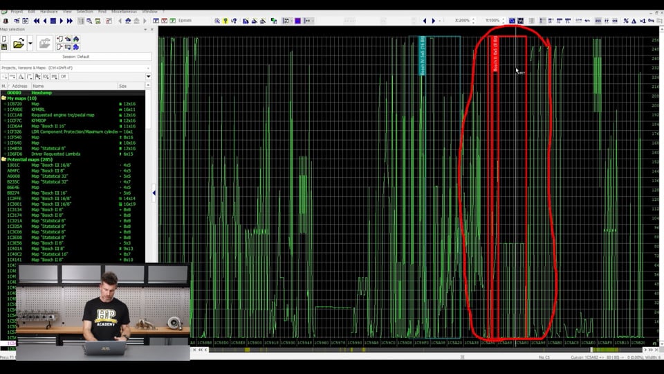
| 08:03 | And then down here, we've got this little folder that says potential maps and it says 285. |
| 08:08 | And if we click on that little folder and open it up, this is all the maps that when WinOLS has found. |
| 08:18 | And these are potential maps within that raw binary file. |
| 08:23 | Now it seems like it might be useful to a degree and a lot of people think when using WinOLS that it's going to do all of the hard work, we're going to open a file, create a new project in OLS and it's going to go through and find all of the maps that we need. |
| 08:40 | Sadly, that is not always the case. |
| 08:44 | When we first open a file, it does what's called a background map search and it's basically looking for patterns in the file that could represent a map. |
| 08:55 | So we can see over here, this is a 2D view and we can see that WinOLS has highlighted this area in the map here, I'll click on it, and it thinks that this might be a map and it's said that it is an 8x5 and it is an 8 bit map, great. |
| 09:15 | It probably is something, however, there could be, in this case, 285 maps that it's found. |
| 09:21 | That is almost certainly complete overkill. |
| 09:25 | If we're doing a basic stage one style tune where we've got a car that's mechanically still stock and maybe it's got an air filter, maybe an exhaust system and we want to raise the boost pressure a little bit, tweak the fuelling and the ignition timing to optimise those, we're probably going to need a handful of tables at best, maybe 10 or 15 tables at the absolutely most, probably actually much less than that so 285 is definitely overkill and this is what's easy to overlook with a factory ECU is they are incredibly complex. |
| 09:58 | There'll be 100s if not 1000s of different parameters and tables and the majority of those we are absolutely not going to need to concern ourselves with. |
| 10:07 | So the fact it's found 285 maps, is straight away overkill and potentially just confusing to us. |
| 10:14 | Just as importantly though, and this is a bit more problematic. there's a pretty good chance that OLS will not find some of the maps that we actually are interested in so this means that it's still on us to actually do a lot of the hard work and actually find these maps. |
| 10:31 | The other element is that even when we find the maps, which we'll see shortly, they by default don't make any sense, the numbers will not look like lambda targets or ignition timing values for example. |
| 10:46 | So we still have to figure out what map we're looking at and then we're going to need to apply some scaling or factors to the raw numbers in order to convert them to something that we're then capable of actually reading, understanding and manipulating. |
| 11:02 | So again all of this will hopefully make a little bit more sense as we go through this but at the moment we're viewing in what's call 2D mode. |
| 11:12 | So I've just circled this down here. |
| 11:14 | We can view our binary file or our maps in text, 2D or 3D. |
| 11:18 | So if we convert to text view, and let's just make this a little bit wider for the moment. |
| 11:23 | This is kind of what we're faced with and it looks a little bit like staring into the matrix. |
| 11:29 | And on face value, particularly if we're looking at it like this, it's going to be hard to do anything remotely useful but hopefully at this stage you're sort of getting the idea that compared to commercial reflashing software, this is a very very different animal and it absolutely is. |
| 11:47 | What I'm going to do for a moment is just close down our potential maps folder because we've got a lot of stuff going on there and that's not overly useful. |
| 11:56 | Let's just have a bit of a tour of what we're looking at here. |
| 12:01 | So on the left hand side, we've got what we've already had a brief look at, the maps that we've found as well as the potential maps. |
| 12:09 | We can also hide this away to give us a little bit more screen real estate if required. |
| 12:14 | Which can be quite helpful depending on the task at hand. |
| 12:17 | On the right hand side, we've got the contents of our binary file and at the moment we are displaying these as I mentioned in a 2D format. |
| 12:25 | We want to do this while we are looking for maps because what we're doing is we are using pattern recognition. |
| 12:34 | So if we're looking for a specific map, particularly when you're just getting started, and this is what we've done within our course is we've provided a sample. |
| 12:42 | For example a lambda for component protection map is going to look a certain way, let's actually have a look at that, we'll click on our LDR component protection map. |
| 12:51 | So, that's actually not the one that I wanted. |
| 12:54 | This is essentially a maximum load table. |
| 12:58 | So this pattern here, I've got one of them that is defined and we're going to define the rest as we go. |
| 13:05 | So this repeating pattern here, this, once we're familiar with it, we know that when we see this, this is our maximum cylinder fill tables. |
| 13:16 | And once we've seen that pattern, we've found that pattern, then we can go ahead and actually define each of the individual maps within this. |
| 13:23 | Another point that is relevant here is that with the factory ECUs, for many of the tables that we're going to need to find and define, there will be multiple variants of those tables. |
| 13:35 | So in this case we've got one, two, three, four, five and six of these maximum cylinder fill tables. |
| 13:48 | In some ECUs we may have much more than this as well. |
| 13:51 | How the ECU processes which of these to utilise is going to be dependent on a number of factors. |
| 13:57 | In a lot of ECUs it will only use one and the other tables won't be utilised at all, it's very very dependent on the specifics of the controller that we are working with. |
| 14:10 | So let's just continue on our little demo here before we get too deep into the weeds. |
| 14:16 | Down the bottom of our screen here, we've got this little bar that shows us where abouts we are in the binary file. |
| 14:26 | So you can see here, we've got a little white cursor, it's turning red as I go over it, that's showing us our current location and directly below that, we can see in the toolbar, it says cursor and then it gives us an address, in this case 1CF340. |
| 14:45 | That is the current address that we are accessing and the value at that point is to the right, it says 5462 which is a meaningless number to us but that's what the contents of that particular location are. |
| 14:59 | So when we first open a file, we're going to be faced with something that looks probably a little bit like this, we're going to be all the way across at position zero, very start of our binary file. |
| 15:13 | So if we just look at the little bar at the bottom here, what we can see is that over on the right hand side, we've got this block of colour. |
| 15:23 | And this is our actual calibration data so all of the other stuff before this, depending on how we've read from the ECU, will contain maybe immobiliser codes, a whole bunch of stuff that's essentially irrelevant to us as it pertains to tuning. |
| 15:40 | So we want to start by actually getting ourselves to the data block that we care about. |
| 15:45 | So we can do that just by holding down and dragging ourselves across there. |
| 15:49 | Then we can manipulate how we, where we are located in this data. |
| 15:53 | Essentially if I left mouse click to the right hand side of the current cursor location, what we're going to do, is we're going to jump forward one screen at a time. |
| 16:03 | If I click to the left of the cursor of course we go back the other way. |
| 16:06 | And hopefully as I'm scrolling through this, you're sort of thinking to yourself much the same way I did when I first got started, what on earth is this, how are we supposed to make sense of it but it really does all come down just simply to pattern recognition. |
| 16:22 | Understanding what we're actually looking for and this also comes down to understanding the controller that we're dealing with. |
| 16:30 | So as I mentioned, this is a Bosch MED 9.1.5, admittedly in this day and age, it is an older controller and it is a little bit simpler than the modern controllers but understanding the logic flow of how that controller works, which without going too deep into the weeds with it, basically it starts by taking the driver's accelerator pedal position and it converts that into a torque request which is actually a relative torque request, a number between zero and 100%. |
| 17:00 | Once it's got that, it then converts that into a requested cylinder fill and then basically that feeds into the boost pressure targets that the ECU is going to request in order to get that cylinder fill. |
| 17:13 | So it's again a little bit different to a standalone aftermarket ECU and as I mentioned, all OEs sort of have their own best practice ideas on how they want to control fuel and ignition so it is a case of understanding for the specific ECU or vehicle that you want to tune, how did the manufacturer of that vehicle decide they wanted to control fuel and ignition because that drives what maps will be available and then that in turn drives what maps we are going to need to find and then we use our pattern recognition in order to find those maps. |
| 17:51 | Now also up the top here, just highlight a few bits here, the top toolbar, we've got the ability to manipulate how we are viewing the data. |
| 18:03 | So we can see we can zoom our X and Y axis, so we're zoomed at 400% at the moment, let's click, that's interesting, there we go, it's working finally. |
| 18:15 | We can zoom in or out to suit, obviously when we're zoomed right out, we get a lot less detail but it does make it a little bit easier to find a particular map shape within the entire binary file when we're first getting started. |
| 18:28 | Once we're actually working with that particular map we may want to zoom in a little bit more. |
| 18:33 | We've got the ability to turn that background grid on or off. |
| 18:37 | Also a bunch of controls for the look and feel of OLS and how it works. |
| 18:42 | So we can change the colour schemes to suit our own personal requirements. |
| 18:45 | Then we've got the ability to work in 8 bit, 16 bit, 32 bit or floating point depending on the data that we're looking at. |
| 18:55 | We are currently in a 16 bit system and that also gives us the ability to set whether it is a low high arrangement or high low which means which of the bytes of data is the most significant bit. |
| 19:12 | Little bit probably familiar to those who have done any CAN bus reverse engineering. |
| 19:17 | We can also display as a signed or non signed table or data. |
| 19:23 | For example if we are looking for ignition timing values, these will be signed values. |
| 19:29 | Then to the right of this we can display as decimal, binary or hexadecimal values. |
| 19:38 | Alright so let's jump into a table and see a little bit more about what this all looks like. |
| 19:45 | So what I'll do is I'll click on the left hand side here and the particular table that I've just clicked on is called KFMIRL. |
| 19:53 | Pretty meaningless and what you're going to learn more than you ever wanted to about is Bosch naming acronyms. |
| 20:00 | If you're using OLS and you want to work with any of the Bosch controllers. |
| 20:03 | Awkwardly they are all derived from technical German and particularly if you buy a map pack for a particular controller, often all of the names and all of the information will be in German. |
| 20:18 | I'll talk about what a map pack is shortly. |
| 20:22 | But let's have a look at this particular table. |
| 20:26 | So we can see here, everything's highlighted and it's given us our name, KFMIRL, it's telling us that this table is 11x16 so that's the size of the table, 11 y axis, 16 wide is our x axis and it is 16 bit values. |
| 20:42 | Looking specifically at the data, what we've got is here, what I've just highlighted, this is the table values. |
| 20:53 | So that's essentially our Z axis, the data that's going to go in the table. |
| 20:57 | Then to the left of this, we've got two axes here, so our x and our y axis and I've just highlighted those. |
| 21:07 | So this one has already been defined so let's just double click on this and we'll have a look at it. |
| 21:12 | And now it's kind of looking a little bit more like what we'd be familiar with with a aftermarket, sorry a commercial reflashing package. |
| 21:22 | We've got the name of that particular table, requested cylinder fill and what we've got here is obviously on our x axis, should be pretty clear we've got our engine RPM. |
| 21:35 | So 500 through to 6500 RPM. |
| 21:37 | The vertical axis here is our accelerator pedal position or driver's pedal position. |
| 21:44 | And then the numbers inside of this table are our requested cylinder fill in terms of a percentage. |
| 21:53 | That's fine but this isn't what it looks like when we first find that table. |
| 21:59 | So if I press escape, it comes back to this view, this is what we're really starting with. |
| 22:03 | Or, if you want to go a little bit deeper, we can actually view this as text. |
| 22:08 | So this is what that table looks like in text view. |
| 22:13 | So again, not really a lot that we can take from this, if we look at the specific values here, we're talking about a value of 60,000 in the table perhaps, depending on where we are. |
| 22:24 | And then we've got our axis values here, so we can sort of see those numbers there, again not really something that makes a lot of sense. |
| 22:33 | Let's come back to our 2D view and we'll double click on this table to get back into it. |
| 22:38 | So before we actually add scaling data to this, if I come over here and I hover over the ignore factor symbol here, this is what the data looks like as we first load it up. |
| 22:57 | So we can see that our x axis, which you'll remember was RPM, is now values of 2000 through to 26,000, not super useful. |
| 23:07 | Our vertical axis which is our throttle position, 427 through to 66,400, again not particularly useful and the numbers in the table are up to 60,000 or thereabouts. |
| 23:18 | So it's difficult initially, until you're used to this, to actually understand what these table axis and values mean and how to actually represent them in terms of numbers that actually make sense. |
| 23:32 | So let's have a quick look at this, we'll go a bit further with this as we go. |
| 23:35 | What we can do is double click anywhere in this table, if I double click right here, I've just hovered over the actual Z axis or data so I'll double click on that with the left mouse button and that opens up the properties box, so straight away it jumps to the axis that I have double clicked on. |
| 23:53 | So see at the top here, we've got tabs for map, for x axis and Y axis. |
| 23:58 | I clicked on the map, so that's what it has opened up. |
| 24:01 | So we can see we can give the table a name, KFMIRL, the description of this is our requested cylinder fill, we can give it a unit, in this case it would be percent. |
| 24:15 | It's then got the start address for this table. |
| 24:20 | It has defined this as a 16 bit arrangement data organisation in high low organisation. |
| 24:27 | And then the important part down here, is that we have this equation which converts our raw value into something that we can make sense of. |
| 24:38 | So what we can see here, if I just highlight this a little bit more thoroughly, we've got the value that we're going to display is equal to this factor, in this case 0.0023438, don't worry about that, I'll talk about that in a moment, times EPROM which is basically the raw value from the EPROM, then divided by one and plus zero. |
| 25:00 | So if we know that factor, we can enter that directly and this is a bit of a tricky one, where do these factors come from? And there's a few different answers here unfortunately, it's not all cut and dry. |
| 25:14 | A lot of this though does come down to understanding the patterns that exist for the numbers we're dealing with. |
| 25:24 | So I've just got a little cheat sheet here that I'll open up. |
| 25:28 | So we can see here, for the binary system, we've got this set of numbers that we will see come up time and time again when we are reverse engineering a map inside of a factory controller. |
| 25:40 | So these are just numbers that just continually double, so two, four, eight, 16, 32, we get up to 128 and then at the end of it, 65,536 so these are often factors that go into these values that we can use to help reverse engineer them, factor them and make them actually something that makes sense to us as a tuner. |
| 26:03 | We've got the same for decimal numbers which is 10, 100, 1000, 10,000. |
| 26:08 | We've got 20, 40 and 60, then we've got some non logical numbers as well. |
| 26:15 | I've also for our course presented some of the common conversion factors for some of the common known Bosch tables as well just to make life a little bit easier but it's just a case of understanding these numbers and then learning how to apply them. |
| 26:31 | So for example, let's have a look at our x axis, so two ways of doing that, I just clicked on x axis, the tab here at the top but we can also close this down and double click on the axis. |
| 26:43 | I actually recommend when you're getting started that this is how you use OLS. |
| 26:48 | Because it makes sure that the axis that you're about to edit is the one that you're interested in. |
| 26:54 | Rather than starting out on the x axis and then manipulating your way around using these tabs, very easy to make a mistake. |
| 27:03 | So let's have a look at this and we'll just get our raw values back. |
| 27:07 | Which we can see again, 2000 out to 26,000. |
| 27:12 | Now you're obviously not going to understand this when you're doing your very first task with OLS but when we see a number of 26,000 in an MED9.1 controller, this is generally a bit of a lightbulb moment because that is a number that I would recognise as being most likely RPM. |
| 27:32 | Also it makes sense because I know what this table should be, so I know that it's going to contain RPM but we need to factor this. |
| 27:41 | So looking through this, we've got our engine speed, we've got the fact that the units there are revs per minute, the data organisation, 16 bit high low, this is a 16 bit table, that is correct so it really comes down to our factors here. |
| 27:57 | So in this example, we would know that the factor to use here is to either muliply the raw value by a factor of 0.25 or divide it by four, obviously the same thing. |
| 28:09 | So we can do that, we can enter a value of 0.25 and straight away we can see in real time the numbers actually change, yep 65,000, ah 6500, probably won't rev our little Volkswagen Golf to 65,000 RPM any time soon but yeah these numbers now make sense. |
| 28:24 | They are a nice smooth progression from a low of 500 up to 6500 RPM, I'm happy with that. |
| 28:31 | The other option here, let's just show you, obviously dividing by four is the same but let's just enter a value of one there, gets us back to the raw value and down here we can see we've got this little function button, we'll click on that and now what we can do is click on the output radio button, which just gives a little bit more control, it's essentially achieving the same thing but now it gives us access to enter a value here on the bottom of the equation of four, you can see that that shows us what the result will be, the factor is going to be 0.25, happy days, we'll click OK, our job is done there. |
| 29:09 | So this is what we're going to be doing while we're going through and finding and defining these maps, this is just one I wanted to give you a quick look through, we'll press escape to close that down. |
| 29:21 | And let's actually start and go through the process of defining a map and I'm going to start with something that is relatively easy which is our LDR component protection maps, which we already had a really brief look at accidentally. |
| 29:36 | So let's have a look at these. |
| 29:39 | I'm going to start with these because they're a little bit simpler because they are a 2D table, 16 bit table and we've got this first one that is already highlighted so how this works, let's get away from that one, we've got two pieces of information. |
| 29:55 | The bit that I'm highlighting here, this is actually the map data and then the other piece of information, this here is our axis for that particular table. |
| 30:06 | So in this case, each of those tables has its own axis, so let's have a look and see how we could go about defining one of these tables. |
| 30:15 | So what I'll do here, I know that this area is our axis. |
| 30:21 | And what I'm doing is I'm just clicking on that axis. |
| 30:24 | And I want to look at the value that it shows me at the cursor position so at the moment we can see that that is a value of 9000. |
| 30:32 | What I'm going to do is just click to the left and we see that drops down and I'm looking for a minimum value there before it jumps back up. |
| 30:40 | That minimum value is 16. |
| 30:44 | OK that's important, what that is telling us is that the axis is 16 long. |
| 30:51 | And the first number to the right of that value of 16 is going to be our first axis value. |
| 30:57 | So now we know that we're looking at a 16 x 1 table, a 2D table with an axis that is 16 long. |
| 31:05 | And if we click on this again, we can see that the one that is already defined is showing us that it is 16 x 1. |
| 31:14 | OK what we need to do now in order to find this table is set up WinOLS so that it is set with a width of 16, down here in the bottom right hand corner we can see that it already is, that's more good luck than good management. |
| 31:31 | We can manipulate this by using the M key to add more width, so I'll take that up to 20, the W key will shrink that back down. |
| 31:40 | This right now is going to seem meaningless but when we jump to our text view it will make more sense. |
| 31:47 | So what we want to do is make sure that we've matched the width that we're operating OLS with to the size of the table, in this case 16, so our job is done there. |
| 31:56 | Now what I'm going to do is I'm going to define our next map across to the right which is the one I've just circled here. |
| 32:03 | What we want to do now is get our alignment correct before we do this and what we want to do is hold down the control key and use our cursor keys until this vertical line that is currently displayed here disappears so let's do this, I'll hold down the control key, use my right arrow key, let's actually go the other way. |
| 32:23 | OK see that that now has disappeared so now what this means is my orientation, my alignment is correct, the first value in the map data here is going to be at the very left of my table. |
| 32:35 | So now that I'm ready to actually define this map, what we can do is just click anywhere to the left of that map data, hold down the left mouse button and then just drag across to the right so that we're basically covering the area of the map that we want to define. |
| 32:50 | Now what we'll do is we'll move to the left hand side of that grey area, and just look at what happens to the cursor as I get to the edge, see the cursor actually changes shape. |
| 33:00 | So now what I can do is hold down our left mouse button and we can drag that back across until we get to the start of our map data, job done. |
| 33:09 | We now want to repeat that on the right hand side so again the cursor changes shape, we'll hold down our left mouse button, drag that back across so now what we can see is we've only got the actually map data which is the bit we're interested in, highlighted. |
| 33:22 | So now we can mark this as a map and we can do this by pressing the K key. |
| 33:27 | Now it's opened it up as a 2D table but I prefer to view this at the moment in text view. |
| 33:34 | So there we go, we've got our table already defined and what it, well table is defined. |
| 33:39 | And what it's already done, because the table before it which shares basically the same configuration, we'd already gone ahead and defined the RPM axis, it's actually sort of looked and gone to itself, you know what, this looks exactly the same as the table to the left of it so it's applied that same factor and scaling but not to worry, if we come up here, this again will be what we'd be looking at. |
| 34:05 | So a value of 27,200, we know that that is most likely going to be our RPM axis. |
| 34:13 | So let's double click on this. |
| 34:16 | So RPM axis, we've got engine speed and revs per minute already entered and it has already applied that scaling as I mentioned but basically the same as what we just did, it would have originally looked like this and we know that in Bosch MED, our factor is going to be divide by four or multiply by 0.25, so that is how we'd go about doing that. |
| 34:39 | Alright so that's defined our x axis. |
| 34:42 | The numbers in the actual table are our relative cylinder fill. |
| 34:47 | So let's open that up and have a look at it. |
| 34:49 | We can give this a name and I think this one is LDR component protection. |
| 34:59 | Really important to try and be consistent with your naming strategy as well so that first of all when we're starting to put maps into folders, which I'll talk about in a moment, it's very easy to automatically populate your folder with all of your maps and also between different controllers or different files, everything remains the same. |
| 35:20 | So what well do is give control A, we'll copy, we'll highlight all of that, control C will copy it to the clipboard, tab will jump down to our description and control V will paste that in. |
| 35:34 | So the values in our axis here are our relative cylinder fill, this is a percentage. |
| 35:39 | And we come down here to our factors. |
| 35:43 | So this is another one of those ones that's a little bit tricky. |
| 35:47 | There is two ways of doing this. |
| 35:49 | The actual factor which would come from a Bosch description file. |
| 35:54 | A description file is essentially a file that Bosch make on each of their controllers and it tells you exactly how the logic flow works, it'll have addresses for all of the maps, the size of the maps, scaling factors etc. |
| 36:10 | So in this case it's 0.023438 and that gives us our values in percentages. |
| 36:18 | We also probably want to add a little bit of precision here so we can come down to our precision and let's add one decimal place of precision. |
| 36:27 | OK so that's one way of getting that number. |
| 36:31 | However this actually also follows, if we come back to our little notepad here, our non logic numbers here. |
| 36:38 | This will get you really close as well and sometimes can be easier to remember. |
| 36:42 | We've got this value here of 42.6. |
| 36:45 | So this is a non logic number that we know is often used as a factor. |
| 36:49 | So let's just scale this back to one, we'll come back down to our little function button, click on that and now let's try dividing by 42.6 and it's not pinpoint accurate. |
| 37:03 | We can see that the resulted factor is 0.023474 so probably for all intents and purposes we're out by a percentage point, it's not going to be that big of a deal but the actual factor for that is 0.0234, 0.023438. |
| 37:25 | Job done there, that is our LDR component protection table defined. |
| 37:31 | Let's press escape and we've still got that marked so we want to press delete and now we've got two of these tables that are properly defined. |
| 37:40 | I'm just going to go through this next one really quickly. |
| 37:43 | So the process is the same, we've got our width still set to 16 obviously. |
| 37:48 | What we want to do is get our alignment correct here, get rid of that vertical line, so control and our right arrow does that, we're going to left mouse click, drag across that, we want to then come to the left hand side, drag that to the start of our map, come to the right hand side, drag that to the end of our map, K key. |
| 38:08 | Oh that's handy, let's just try that again. |
| 38:21 | Third time's the charm. |
| 38:28 | Right get that to the correct location and now it's created a map from that, we'll come back to our text view and again it has found the scaling for our engine RPM axis but it hasn't done that for our z axis, our map data so let's press escape, press delete. |
| 38:47 | And the other thing we can do here is actually copy the scaling data, the descriptions, the IDs etc from one map. |
| 38:58 | Because as you can imagine there, we've got six of these maps, it's going to get pretty tedious, pretty time consuming if for each of those maps we define we have to manually enter the scaling factors, the names of the axis etc so what we can do here, let's go to our first one which I actually didn't do live here. |
| 39:15 | We'll right click this and what we want to do is copy map properties. |
| 39:22 | So I'll click on that, now we have to define what we actually want to copy. |
| 39:25 | So in this case, not a lot, all we want to really do is copy the description, the name, description, the factor offset precision etc and where do we want to copy that from? Well we want to copy that from the x, the y and the z axis. |
| 39:40 | Obviously we don't have a y axis for this but that's OK. |
| 39:43 | Do need to be a little bit careful with copying map properties because we can see I've got this other box out here. |
| 39:50 | And at the moment I've got this little tick box ticked here for data source plus address. |
| 39:55 | I don't want to do that for what we're trying to do here. |
| 40:00 | We'll see how that plays in shortly. |
| 40:02 | So we'll click OK, so that's copied the map properties. |
| 40:05 | Now if we open the next map up and control V, that will now apply all of that. |
| 40:11 | So hopefully what you actually saw was our name change because it was slightly different between the two maps. |
| 40:17 | So job done there. |
| 40:18 | Let's open our third map up, control V and watch the data inside of the map change as I apply the scaling. |
| 40:26 | There we go, job done. |
| 40:27 | So much much quicker way of doing it and what it's also doing here on the right hand side is we can see that it is starting to add these maps in over there so we can see all of the maps as we define them. |
| 40:40 | We'll do one more and I'm going to go about this a slightly different way and first of all I'm going to just change our width, I've talked about this width before, you can see, I'l just actually draw over the top of it. |
| 40:52 | You can see that it is currently 16. |
| 40:54 | To show how that affects things, what I'm going to do is just change that out to a value of 20 for the time being. |
| 41:01 | Let's come over here to the right to our next map and we'll just click somewhere near the end of that map data. |
| 41:08 | Now we'll convert to our text view. |
| 41:10 | So, what are we actually looking at here? Well the number that I've highlighted here is a value of 16. |
| 41:18 | And doesn't really make too much sense at the moment. |
| 41:23 | So what we can do here, is look for clues, this actually becomes a lot easier in the next map that we'll look at because it is 3D, very hard to do this technique when we are using a 2D table so bear with me anyway. |
| 41:42 | We know in this case it is 16 wide so let's look at the graphical representation out here on the right hand side and what I'm going to do is I'm going to use the w key to narrow this down from 20 to 16 and we'll see that this all changes shape and we're going to get to, now we're at 16, we're going to get to a point where everything sort of looks like it's got the right shape to it but our alignment isn't correct so we're going to now hold down our control key and we'll go, there we go, so we've got our values now for our table all aligned, let's just press escape here, we'll go to our 2D view. |
| 42:23 | So we can see that we've got everything set up to define this map data here. |
| 42:29 | Let's click on our first value here, we'll get rid of that and we go back to our text view. |
| 42:34 | So we can see this is the first value for our next table. |
| 42:38 | So just a different way of doing this which is much easier in my opinion, particularly when we're doing 3D tables, what I'll do is I'll shift, hold down the shift key, use our right arrow key, that's highlighted that particular table. |
| 42:52 | Now I can press the K key, we've created our map again, let's switch across to text view, control and V and there again we've applied our scaling as well as our description and map ID. |
| 43:05 | So we'll press escape there, delete and we'll get rid of that. |
| 43:08 | Let's switch back to our 2D view. |
| 43:10 | Alright so I'm not going to do the other two maps because it's just a rinse and repeat but what I will show you is how to use folders because that's super helpful. |
| 43:19 | Now as I've already mentioned, a lot of the tables that we will be finding and defining in OLS will have multiple variations of the map and if we were just filling out our maps over here with all of this data, it starts to get pretty confusing and difficult to find what we want, particularly when we get to a point of actually using OLS to tune. |
| 43:40 | So what we can do here is come up to our component protection map, we'll hover over the name, it's important that we are hovering over the name and we're going to right click. |
| 43:51 | And we're going to come down to copy name. |
| 43:54 | So we've done that, now what we're going to do is right click again and we're going to click this time move into. |
| 44:01 | Click on that and we want to select new folder because we don't have a folder at the moment. |
| 44:06 | So control V, we're just going to copy, we're going to paste the name that we've already copied into the name there and then we're going to click on this little box that says if the name contains the following text, and again I'm going to control and V, then apply rule to existing maps. |
| 44:24 | So basically what that's going to do is make a folder, with the same name that we've just pasted and then it's going to automatically move any maps that we've defined with that name into that folder. |
| 44:36 | Plus if we create more maps with that same name later on, it's going to also copy those into the folder. |
| 44:42 | So there we go, job done and now we can see, that we have our LDR component protection maximum cylinder fill folder, we can click on that and that is going to open up and show us the four of the six maps that we've now defined. |
| 45:00 | Alright so that's our first little demonstration, that actually took a hell of a lot longer than I expected. |
| 45:06 | Hopefully this is going to make some sense to everyone. |
| 45:10 | Let's have a look at one more, we'll see how much time we've got, whether we can do a couple. |
| 45:16 | So let's have a look at our next maps that we're going to define and we've got one here that's already defined and it's called requested engine torque pedal map. |
| 45:25 | So again, let's just shrink this down and we'll make this a little bit smaller. |
| 45:32 | So this is another really obvious shape, these maps here which is basically our driver's pedal request, in terms of converting our pedal request into a relative torque. |
| 45:44 | So we can see that we do have a number of these as well. |
| 45:49 | Now there's a trick with this one though. |
| 45:51 | We can see that the one that is already defined is a 12 x 16 map but we can't see any axis values here, there's certainly nothing to the left here and if we scroll across to the right, probably should have shrunk this down a little bit. |
| 46:12 | But if we scroll across to the right, it will happen I promise, let's just go a little bit quicker. |
| 46:19 | What we will find is that the axis data is actually at the end here so that's this blue area that is also highlighted out here. |
| 46:30 | So differences compared to what we've got there, no longer do we have a set of axes for each map. |
| 46:38 | All of those maps share the same common axis and also obviously the axis is at the end of the map instead of at the front so a little bit different there to what we're used to but we can work with this. |
| 46:51 | So let's have a look at how we can go about defining one of these maps and what I'll do is just make sure that we aren't aligned properly at the moment. |
| 47:02 | We'll come to the end of one of these maps. |
| 47:09 | And we want to just click somewhere near the end, doesn't have to be too precise at the moment. |
| 47:12 | So let's convert to our text view and now I'm going to show you what I was trying to show you before which is utilising the graphic off to the side to help with our alignment. |
| 47:27 | So initially we cheated here a little bit because we've already got one of these maps defined but normally we wouldn't know by looking at this necessarily what the map size is in terms of how many x and y data points we've got. |
| 47:42 | So what I'm going to do here is I'm going to use the w and m, w shrinks everything down, m adds and we've got our width currently set to 17 and what we want to do is essentially change this until everything starts to align so let's just press the w key. |
| 48:01 | OK so what we're starting to see here, what I'm looking for is this line that's on a bit of an angle at the moment. |
| 48:11 | When we've got our width set correctly, that is going to jump to a nice vertical line so let's go a little bit further, we'll press the w key again and straight away we've now got it lined up vertically so we can see that vertical line through there, this is telling me that I've got my width correct now and the width down the bottom right hand corner is saying 12 so that's going to basically line up with one of the axes, will be 12 x something essentially. |
| 48:42 | But if we actually look at the data, we can see that while we've got that vertical line through it, the data doesn't make much sense because if we look sort of from, let's say from left to right as we go across here, it sort of starts really low then jumps up and then dives away to nothing again. |
| 48:58 | So what that means is we still haven't got our alignment quite correct so if we hold down the control key and use our left and right arrow keys, now what we've got is something that actually makes a bit of sense. |
| 49:10 | Alright so let's see how we can now use this to define our table. |
| 49:16 | So looking at this, our top value here is zero and then the pattern repeats so basically one table is everything that I've just highlighted here and you can kind of see that this pattern then repeats and repeats with each of the tables. |
| 49:34 | So we know that zero is our top left value and what we're going to do is come across 11 for a total width of 12 and then we're going to come down here, three, four, five, six, seven, eight, nine, 10, 11, 12, 13, 14, 15, 16. |
| 49:49 | so we're looking at a table that is 16 x 12. |
| 49:53 | So if I press the K key that will mark that and turn it into a table, let's have a look at it in text view. |
| 49:59 | Alright what do these numbers mean? How can we scale them? So at the moment for a start we can see that our y axis is 0-15 and our x axis is 0-12 so not useful for us but that's alright, we'll make sense of that shortly. |
| 50:15 | First of all what we want to do is scale this particular table. |
| 50:19 | So this comes down to understanding what this table is going to mean. |
| 50:24 | It is a driver's wish or driver's requested torque table. |
| 50:29 | So we know that one axis is going to be our throttle position or accelerator pedal position. |
| 50:34 | The other axis is going to be engine speed. |
| 50:37 | The data here is going to be relative torque request. |
| 50:41 | So in Bosch this is not a specific newton metre number as I mentioned earlier, this is a requested torque, relative torque value 0-100%. |
| 50:51 | Might sound like a weird way of doing it but the reason that Bosch do it like this is that the same exact controller logic can be used in a four cylinder naturally aspirated engine or a V8 twin turbo, it doesn't matter. |
| 51:07 | 100% relative torque is still 100% relative torque, even if the specific torque in newton metres is going to be dramatically different. |
| 51:15 | Alright so that is the tip though, we know that this table is going to be representing a value of 0-100 and if we look at these values here, at the top, 32,768, now that's not something that's necessarily going to make much sense but let's have a look at our little cheat sheet and if we go through this row of numbers we can see that 32,768 is in fact one of our binary system values so this is a common factor. |
| 51:46 | Let's close that down and we'll double click on our axis and this will be driver's wish. |
| 51:56 | And we can copy and paste that. |
| 52:01 | I'm just going this reasonably quickly here, I would normally be a little bit more thorough with my naming strategies and what we want to do is come down to our factor and in this case we want to use the divide by so we're going to click on our function button, we'll click on our output here, I'll just drag this out of the way so we can see the whole table. |
| 52:21 | So we know that our value is 32,768 so let's enter that. |
| 52:27 | OK so that gives us down to one which is pretty straightforward if we divide a number by itself, of course we're going to get one. |
| 52:33 | But we want a number up to probably 100 so this just means that we need to put our decimal point in another place and if I remove the 68, we're now 327 and we can see the numbers in this table are now ranging up to 100 so yeah we're probably on the money. |
| 52:49 | While it's splitting hairs, we still need to use the entire factor so we enter a decimal place, 0.68, job is done. |
| 52:59 | And if we wish we can add some precision here to this with a decimal place. |
| 53:03 | So this is how using the factors, those binary factors, the scaling factors, and also just having an understanding of what the table is actually trying to tell us, can make it really really quick and easy to actually define this, even though on face value these numbers are just absolute garbage. |
| 53:22 | Now let's close that down for a moment because we still need to find our axis values. |
| 53:27 | So let's have a look at this in 2D view. |
| 53:31 | And we know that our axis is out here. |
| 53:37 | So let's just scroll down, what I'll do is I'll show you what I'm doing rather than doing it myself and not making any sense. |
| 53:44 | So we know that the axis values are here. |
| 53:49 | What we want to do is basically find the address of those axes. |
| 53:53 | So I've clicked on one of these axes, so we can see the shape is like this. |
| 53:59 | And again I'm looking at these numbers here to the right of the cursor. |
| 54:03 | So if I go to the left, I'm going to get to the lowest value here, there we go, 12. |
| 54:10 | So this is the axis that is 12 long and the first number to the right of that is our first axis value. |
| 54:18 | Now if we scroll across here, our next axis is going to be of course this one here, so we can basically do the same and I'm going to expect that this is going to be a value of 16. |
| 54:30 | There we go, right there. |
| 54:32 | So this tells me that we've got our two axes, one 12 long, one 16 long. |
| 54:37 | Let's have a look at this in text view, I'll leave the cursor there and it shows us where we are. |
| 54:42 | So this is our 16 long axis here, so we can right click, we can come across to the first value here and what we'll do is also just get our alignment right so our width at the moment is 12, just so I can show you how this works. |
| 54:58 | We know that this however, this axis is 16 long so what I'll do is I'll just add four, so our axis is the right length and then what we'll do is use the control key and scroll across so that the first value is on the far left side and now what we can see is that the little graphic on the right hand side shows a nice consistent shape so we know that we've got that right. |
| 55:21 | So what we can do here is one of two things. |
| 55:24 | What we could do is right click here and we could go copy address and then we could go back to our map and we could paste that in. |
| 55:34 | Or alternatively what we can do is we can come down here, we can actually directly define this as the address, as the x axis of the previous map or the address as the y axis of the previous map. |
| 55:45 | Now I don't actually remember which way around this was so let's just have a look. |
| 55:49 | We are, 16 is the y axis so let's go back to that. |
| 55:53 | And we'll right click, address at y axis. |
| 55:59 | So now if we double click on this, we can see we've now got the axis values correct, they are consistent, they're making sense, we'll come back and scale that in a moment. |
| 56:09 | We've still got our RPM axis to do which we can see there is 0-11 which means that it is 12 wide. |
| 56:17 | So let's have a look at that, we have our axis here 12 so the first value to the right of that is going to be our first RPM value. |
| 56:28 | We can right click on that and set that as address at axis of the previous map, let's double click on that, job done. |
| 56:37 | Alright let's quickly define this and we'll show one more example of how we can copy the map properties. |
| 56:44 | So for our engine speed axis let's call that engine speed and again it is going to be RPM. |
| 56:51 | It's probably a good time to mention if you've got any questions, we'll go into Q&A shortly so please start asking those. |
| 56:59 | And our factor for our RPM is 0.25 so yep out to 6000, interestingly depending on which specific map, you'll have seen that some of these go out to 6000 RPM, some out to 6500, some out to 6520 but obviously there'll be reasons why Bosch decided to do that. |
| 57:20 | Our y axis, now again this is understanding what we're looking at here and what the map should be. |
| 57:27 | Remember I said that the axis will be accelerator pedal position by RPM so we know that this y axis is there for accelerator pedal position. |
| 57:36 | What's that value likely to be? Well probably 0-100 would make a bit of sense wouldn't it. |
| 57:41 | So let's have a look at or maximum value, 65,535. |
| 57:46 | Let's have a look at our factors again. |
| 57:49 | Well what do you know, the last factor there is 65,536. |
| 57:53 | Now you're probably saying to yourself, but that's one different to 65,535 and you'd be absolutely correct. |
| 58:01 | The bit that you don't want to lose track of is that there are 65,536 values but the first of those is zero so we're not actually counting from one, we're counting from zero, that explains why we have a difference of one. |
| 58:16 | Alright let's scale this anyway. |
| 58:19 | We'll again use our little function icon. |
| 58:24 | And 65, so I've entered 65, we can see that our maximum value is still 1000 so we need to add another number, 65,500 and then we'll enter a decimal place, 0.36, job done, we've now got zero through to 100, we'll click OK, if you really want to, you can add a little bit of precision to that, it's probably going to make absolutely no difference there and that axis is driver's pedal and of course we are percent. |
| 58:55 | Click OK job done. |
| 58:57 | Alright so that is the process we go through. |
| 58:59 | I have done this reasonably quickly, obviously we've only looked at a couple of maps, some are simpler, some are more complex than what we've looked at so there is a lot to learn. |
| 59:08 | This is definitely not a software package that is going to take five minutes for someone to pick up and go running with. |
| 59:15 | Let's just have a look at one more element here though, so we'll right click here and we want to copy map properties so we'll show how we can use this to then create the next map in this series. |
| 59:28 | So what do we want to do here? Well we want to do what we did before, we want to copy the name, description, factor and offset. |
| 59:36 | We also want to do this from the x, y and map axes but you'll remember that this time we've got one address for our x axis and one address for our y axis and that is shared amongst all of those maps. |
| 59:49 | So this time we want to come over to our data and we want to click here on our data source plus the address, that's really important, and we want to make sure that we are copying that from only the x and y axis, we don't want to copy the map data, otherwise it'd be the same. |
| 01:00:06 | Alright so we click OK and that has done exactly that, we'll close that down and now what we can do is get our alignment back to 12. |
| 01:00:18 | And we'll just get ourselves set back up here. |
| 01:00:21 | So we can really easily see this kind of trend here on the right hand side graphically that represents where the next map is. |
| 01:00:30 | What I'll do is I'll actually jump out of order here, and I'll do this one up here because hopefully, WinOLS is going to actually make our life a little bit easier here. |
| 01:00:39 | So let's come up to this one, we know that our first row is zero because when we're at 0% throttle we're obviously not requesting any torque so we'll come across here, come across 12 and come down 16. |
| 01:00:53 | And that is our table highlighted, we'll press the k key to mark that. |
| 01:00:58 | Jump to text view, control and v and straight away we can see, it's done all of the hard work for us, those axes have appeared as if by magic and they are scaled correctly, everything's done, escape key. |
| 01:01:13 | Now what you can see is that OLS has done what I hoped, it's actually jumped ahead and it's highlighted this next map down, it's sort of basically said to itself, oh hey I can see some data that looks really similar to what you've just highlighted here so I think this is another map in this range so it's got it right this time, press k, again we'll jump to text view, control and v, job done. |
| 01:01:37 | So this is the process we can go through, again obviously I've only given you a couple of examples of this but hopefully you can sort of see how this all works and how powerful it is. |
| 01:01:49 | Really it is a process of three elements. |
| 01:01:53 | The first is understanding how the base controller works and what this means is if we understand how the controller works we're going to probably have a pretty good understanding of what maps are going to be available in that binary file. |
| 01:02:06 | Then once we know what we're looking for, it's a case of using pattern recognition. |
| 01:02:10 | Now of course to start with, you're not going to know what a component protection lambda target map is going to look like in terms of its shape which is why inside of the course, we've provided sample screenshots of all of the common maps so you can start building that muscle memory of what this particular pattern will look like. |
| 01:02:30 | Then it's a case of locating those patterns inside the raw binary file and then it's a case of defining those particular maps and then adding the scaling. |
| 01:02:39 | Once you've done that, then you're left with something that you can tune essentially no differently to a aftermarket commercial, sorry a commercial reflashing software package. |
| 01:02:52 | Now there are a couple of other elements that I just want to quickly talk about before we jump into our questions here. |
| 01:02:58 | Just as important as understanding what WinOLS is, is understanding what it's not. |
| 01:03:03 | And with very few exceptions, you're not going to be actually performing reading and writing from the ECU using the OLS software package. |
| 01:03:13 | Instead, you're going to need to pair this with a third party piece of hardware to do that. |
| 01:03:20 | So there's a number of these on the market, Autotuner and bFlash would be a couple that we've got access to, we've been using bFlash for the course. |
| 01:03:30 | That interface will also generally allow you to datalog as well which is something that OLS doesn't do inside of itself. |
| 01:03:40 | So once you've basically, the process is to read the file out of the car using your third party piece of software and hardware then you can import that file into OLS, define it, you can then make your changes, once you've made your changes and you're happy with the file, you would then export it back out of OLS to your piece of hardware and then flash that back into the car so there's a little bit of tooing and froing here that goes on. |
| 01:04:05 | The other element is how you go about that read and write process and you can do this via the OBD2 port in most instances but maybe not all. |
| 01:04:16 | Alternatively you can actually remove the ECU from the vehicle, connect some jumpers to the header plug on the bench and do a bench read or a bench write. |
| 01:04:25 | Big advantage with doing this is while there's a little bit more faff involved in physically removing the ECU, what this is doing is a complete read of the entire contents of the ECU and why that's beneficial is if something goes wrong and you happen to brick the ECU, most often if you've got a full bench read, you will be able to recover that ECU which might not be the case if you've done an OBD2 read. |
| 01:04:50 | Nice thing with the OBD2 read and write is it's very quick and it's nice and clean, you don't have to get your hand dirty, you don't have to find the ECU and physically extract that. |
| 01:04:58 | In some instances, and I unfortunately haven't had the displeasure of having to do this yet but we will introduce this into the course at some stage, is what's called a BDM read which is where you physically have to open the ECU up and connect to pads on the PC board and read directly in this manner. |
| 01:05:19 | This is called background debug mode. |
| 01:05:21 | This is a lot more work but in some instance may be your only way and then it gets into the complexities of how to open the case of your ECU and not damage the ECU and then also how to reseal it once you've finished your calibration and make sure that it still remains weathertight. |
| 01:05:41 | Last topic before we get into our questions is checksum errors and checksum correction. |
| 01:05:47 | Not admittedly something that you will usually need to worry about but checksum is essentially a validity check, sanity check that the ECU does, it basically sums up all of the contents of a section of its memory and the total value should equal the checksum and if it doesn't, what it means is that either something's been corrupted or there's been a data transmission error and the ECU knows that there's a problem and generally it'll go into some kind of limp home mode which generally means that the engine won't start. |
| 01:06:23 | So of course, from our perspective any time we're changing the contents of one of these memory locations, we need to recalculate the checksum. |
| 01:06:32 | There's a couple of ways of doing this, you can purchase modules for OLS that will do this for you but most of the tools that you'll be using for reading and writing will do their own checksum correction. |
| 01:06:45 | So it's just important to understand whether your tool is doing that or whether you need OLS to do it because if you don't do the checksum correction, then you are going to be going nowhere fast. |
| 01:06:56 | Alright let's head over to our questions and we'll see what we've got here. |
| 01:07:05 | OK no questions which is great from my perspective 'cause that's going to be nice and quick to answer. |
| 01:07:12 | Either everyone's fallen over and gone to sleep because this was too intense, or I've done a great job of explaining it. |
| 01:07:19 | I'm going to hope it's the latter there. |
| 01:07:21 | Regardless, if you are watching this at a later point in our webinar archive and you do have questions that pop up on this, please feel free to ask those in the forum and I'll be happy to answer them there. |
| 01:07:37 | Thanks for watching and hopefully we can see you again next time. |
Timestamps
0:00 - Introduction
1:24 - What is WinOLS?
1:56 - Defining maps is a very different skillset to tuning
3:17 - How it differs to conventional tuning software
11:56 - WinOLS tour
12:25 - Pattern recognition
14:10 - Current file location tool
15:40 - Moving around the file
17:51 - Map view controls
19:38 - Defined map overview
29:21 - How to define a map | LDR component example
43:15 - How to use folders
45:11 - How to define a map | Driver's pedal request component example
59:15 - Copy map properties
1:01:49 - Map definition process summary
1:02:52 - Pairing with third party hardware to perform ECU read/write
1:04:05 - OBD2 vs bench vs BDM read
1:05:41 - Checksum correction